Introduction to Electronic Amplifiers

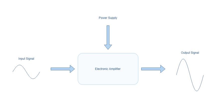
An amplifier is an electronic block that magnifies either potential signals (voltage amplifier), intensity signals (current amplifier) or both (power amplifier). The amplifier consists of two inputs which are the signal to amplify (see Input Signal on figure 1) and the supply of energy (see Power Supply). The output (see Output Signal) is the input signal that has been amplified of a certain gain.

Amplifiers are found at most of the stages of many electronic applications :

• On input stages they bring the signals up to a value where they can be exploited by the circuit.
• On intermediary stages they maintain and correct the magnitude of the signals.
• On output stages they normalize the amplitude to meet standards for the connections.

The main difference between common passive components such as resistors, capacitors or inductors is that an electronic amplifier is an active component since its made of more basics active components. An active component by definition contains internal sources of energy as showed in the following diagrams.

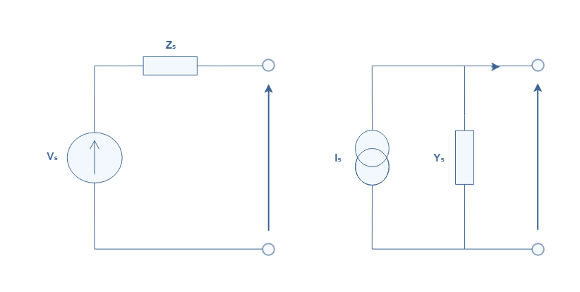
There are two different types of sources : the voltage and current sources. A voltage source provides a constant voltage for a certain range of current. A current source delivers a constant current for a certain range of voltage.

Typical active components used for amplification are electronic tubes and transistors. Historically, the tubes are older and are still used for some specific applications that require high power. Since the 60’s however, bipolar or MOSFET transistors have become cheaper, faster, more efficient and require less supply to amplify signals in most of the daily electronics we use : TV, phone, computers etc …

The quadrupole representation

To precisely represent a voltage amplifier, the Thevenin representation is more adapted since it describes directly the relation between the output voltage and the source. For the same reason, the Norton representation is more adapted for current amplifiers.

If we consider the power supply input to be independent from the input and output signals, we can represent the amplifier according to the quadrupole model :

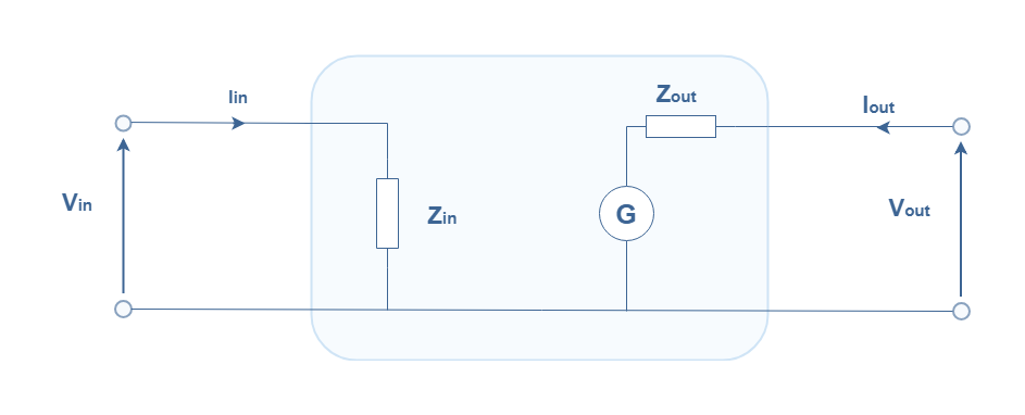
Only four parameters can here fully describe how the amplifier works : the input impedance Z_input, the output impedance Z_output, the transconductance G and the reaction parameter G₁₂. As mentioned previously, the transconductance block G acts precisely as a voltage source. The general relation between these parameters and the signals V_input,  I_input, V_output and I_output is given by the following equations :

Equation 1 : General relations for a voltage amplifier

The ideal model

An amplifier is considered to be ideal when the shape of the signal is not modified by the process of amplification, no matter what is the shape or the frequency of the input signal. Moreover, the gain should be a constant value, regardless again of the shape or frequency of the signal and noises should not be amplified.

When considering the amplifier to be ideal, the output current I_output does not influence the input V_input, hence G₁₂=0. The output impedance Z_output is also considered to be equal to zero in the case of an ideal voltage amplifier since the output current does not influence the output voltage.

The relation between these parameters and the signals V_input,  I_input, V_output and I_output for an ideal voltage amplifier is given by the following equations :

Equation 2 : General relations for an ideal voltage amplifier

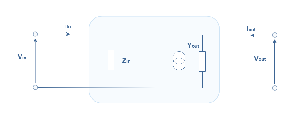
It is easy to find from the equation 2 that the gain (A) of the ideal voltage amplifier can be written as the fraction A=V_output/V_input=G/Z_input. We can note that this model can be adapted to the current amplifier by replacing the output impedance Z_output  by a parallel output admittance Y_output.

Usually, the gain of an electronic amplifier is written in decibels (dB). For example, if an amplifier has a gain of A=10⁶ , we can convert it in dB by using the formula:

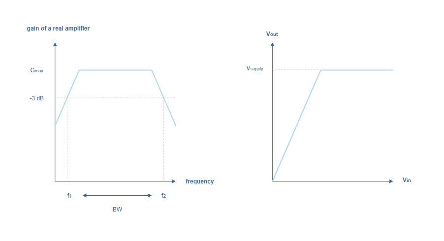
Limitations of real amplifiers

Most of the time, this ideal model can be used for simple calculations. However, ideal amplifiers cannot be built due to physical and technological constraints. Real amplifiers tend to have a constant gain A only on a certain range of frequency f₁ to f₂ called bandwidth (BW). These cutting frequencies correspond where a loss of 50 % to the maximal gain appears. In dB scale, this corresponds to a loss of 10log(0.5) = -3 dB. Moreover as shown in Figure 5, the output voltage cannot exceed the supply voltage leading to a saturation effect of the amplification process.

As we will discuss it more in details in the next tutorial about Common Emitter Amplifier, the supply voltage V_supply controls the flow of electrons in the active bipolar transistors found in amplifiers. The saturation effect precisely occurs when the flow of electrons can not be greater than the command voltage. A good analogy of this phenomenon is a tap water system : the flow of water can not exceed a certain limit set by when the tap is fully opened.

Another limitation to consider for real amplifiers is the distortion of the output signal. Due to intrinsic non-linearities of the active components the output signal can present a different shape than the input signal.Distortions can have many causes, one of the most visual and common type is the amplitude distortion. The cause of this distortion is directly due to the bandwidth (BW) of the amplifier.

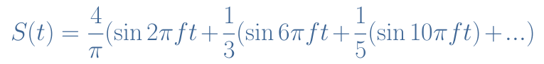
As an example, let’s consider a square signal S(t) of frequency f=10 kHz to be amplified by a limited f_c=50 kHz BW amplifier of maximal gain A_max=10. According to Fourier’s theory, every periodic signal can be written as an infinite sum of pure sine signals called harmonics.

For a square signal, the Fourier serie can be written such as :

An ideal amplifier would multiply all the terms of the Equation 3 sum by a constant value A_max. However, a real amplifier as described previously would indeed amplify the first term and second term sin(2πft) and sin(6πft) of A_max but the third term sin(10πft) would be amplified only of 0.5A_max since this term correspond to a harmonic of frequency f_c=50 kHz. The other harmonics of higher frequencies would be less amplified since the gain of the amplifier continues to decrease (see Figure 6).

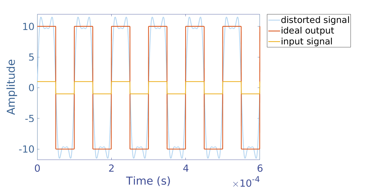
As a conclusion the output of a square signal S(t) amplified by an amplifier of 50 kHz bandwidth and gain A_max=10 would look distorted such as presented in the figure 6.

Mathematically speaking, this type of distortion is equivalent to only keeping the harmonics of the input signal that are under the cutting frequency of the amplifier. The output signal does not remain thus as an infinite sum of sine but becomes a finite sum.

Noise Considerations

The noise N is another undesired effect that often affects electronic amplifier. Many types of noises exist and their cause is never easy to understand and commonly due to the microscopic structure of the semiconductors used in electronic components or quantum phenomena. Their consequences are however very visual since it adds a random parasite signal to the expected ideal output. The ratio signal/noise (S/N) is usually given in dB because on an oscilloscope figure for example, the signal and the noise can simply be substracted since:

It is a quantity that one wants to maximize to get a proper amplification. If the ratio is much higher than 1 (in linear scale) the noise is negligible, if the ratio is close to 0 (in linear scale) the amplitude of the noise is higher than the amplitude of the signal which will completely distort the signal.

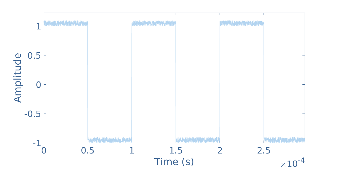
In Figure 7 we can see an example of a square signal of frequency 10 kHz with a noise of 10 % of the signal : S/N=10.

Classes of electronic amplifiers

According to the electronic architecture of an amplifier, to the way that the transistors are interconnected, the purpose of amplifiers and their specifications are different. We can however commonly distinguish four working families and classify them according to the list below. Next to the class name is given the proportion of the input signal that the active components use to realize the amplification process. This concept will be more detailed on the next articles of the amplifier tutorial.

• Class A : 100 % of the input signal is used: The power stage always delivers current (the transistors are always in passing state). The response of the amplifier is thus very fast since there is no delay to activate the transistors. The distortion is very limited but the efficiency is usually low, always less than the theoretical maximum of +50 %. The efficiency is the ratio P_used/P_supply and represents the losses between the power effectively used to amplify and the power supplied to the amplifier. Thanks to these advantages, class A amplifiers are usually more expensive, but very appreciated in the music industry because they can amplify sound without modifying the content.
• Class B : 50 % of the input signal is used: in that architecture, the amplification stage does not always deliver current (the transistors are on stand-by mode). This type of amplifier is thus slower than the class A and presents more distortion but has a better efficiency up to 70 %. Class B amplifiers are cheaper to manufacture since they do not need high quality power supplies to operate.
• Class AB : >50 % and <100 % of the input signal is used: Such as the name refers to, this class is a mix between classes A and B. The amplifier has the capacity to first work has a class A when no or small inputs are applied and can switch to a class B when the inputs increase. Most of the affordable amplifiers for TVs and headphones for example are class AB amplifiers since they can deliver a good output on a wide range of power.
• Class C : <50 % of the input signal is used: This type of amplifiers is used for high frequency application such as in kitchen microwaves for example. Their efficiency is very high (above 80 %) but they generate a lot of distortion.

The class D is known better under the names chopper and inverter. In these architectures, active components (transistors) are used as commutators : they act as a short or open circuit. They are mostly used to control electric engines and they present a very high efficiency around 80 to 90 %. In this class, 0 % of the input signal is used to realise the amplification. More classes that are not mentioned here are available for very specific applications and properties.

In the next tutorial, we will look much closer to the internal architecture of electronic amplifier and more specifically to the role bipolar transistors play. A serie of three tutorial will detail the three elementary configurations of bipolar transistors to amplify signals : the common emitter, collector or base amplifiers.

Please follow and like us: