Kirchhoff’s Circuit Law

Introduction

In this tutorial, we present one of the most fundamental and important sets of laws for electrical circuits. These laws have taken the name and been established by the German physician Gustav Kirchoff in 1845.

Like for many physical laws, Kirchoff’s circuits laws (KCL) are relatively easy to understand and emerge from the observation of conservation of energy, which is probably one of the oldest and most fundamental principles in physics.

Nevertheless, KCL might be simple and accessible to understand, they remain a fundamental tool to master for the circuit’s analysis and are still nowadays widely used.

KCL consists of two different laws relative to the physical values that define the energy in an electrical circuit: the current and voltage. In the following, we separately present in two sections, Kirchoff’s current and voltage laws.

Prior to these sections, it is worth presenting in the first section the framework in which KCL laws are used and many definitions associated with this principle.

The third section shows an example of how to apply KCL to a real circuit and solve a problem with unknown parameters.

Finally, the last section presents briefly the limits of KCL for some particular cases.

Framework and definitions

The framework to apply Kirchoff’s laws is electrical circuits, which consist of a power source or generator with both poles connected with the intermediate of components in a closed-loop configuration. Electrical circuits are drawn according to the lumped-element model, which assumes the components to be ideals, and the associated representation is shown in Figure 1 below:

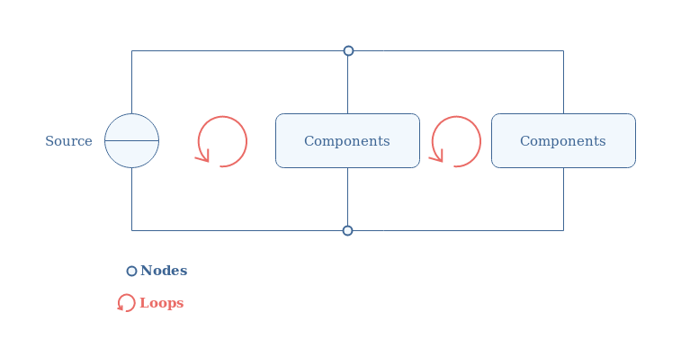
We can give some specific details concerning the topology of the circuits. The straight lines are ideal connections/wires between the different elements of the circuits, which means that they present no resistive or reactive behavior, hence there are no power loss or phase-shift phenomena.

The source provides the circuit with power, which consists of voltage and current signals (either DC or AC). The components are passive, they consist of associations of resistor, capacitor, and inductor. They can either be connected in parallel, such as in Figure 1, or in series. Active components such as amplifiers are not considered in this tutorial since an external source of power is associated with them. A group of components connected at both terminals with wires is called a branch.

Two important topological definitions are important in order to fully understand Kirchoff’s laws later on: the nodes and loops. Nodes represent the junctions between branches, and they are highlighted in Figure 1 by blue circles. The loops are highlighted by red circle arrows in the previous Figure, and it represents a closed path of branches.

Kirchoff current law

The current law is also known as nodal or junction law and states that the algebraic sum of the currents meeting at a node is equal to zero. A simple example can be illustrated with a node connecting three branches:

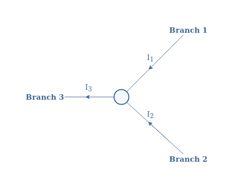
The law states therefore that the sum of the currents entering the node is equal to the current(s) exiting the junction. In our example, this sentence mathematically translates to I₁+I₂=I₃ or I₁+I₂-I₃=0, the current I₃ is negative because it is exiting the node.

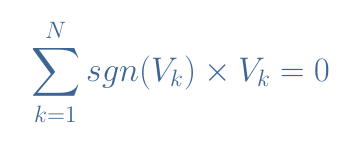
In the general case, a nodal junction of N branches which currents are labeled I₁, I₂,…, I_N satisfies the following Equation 1:

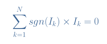
The sign function sgn is equal to +1 if the current I_k enters the node or -1 if it exists it.

The nodal law is directly written from the observation that the charge in a closed system is invariant. This assumption is also known as the charge conservation principle.

Kirchoff voltage law

The voltage law is also known as the loop rule, it is very similar to the nodal rule but applies to loops instead of the nodes. This second law states that the algebraic sum of voltages in a circuit loop is equal to zero. A simple example can be illustrated with a DC source powering a series RC filter:

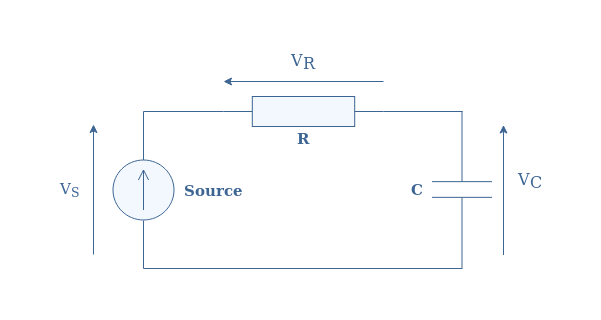
The sign of the voltages is determined with the direction of the arrows, usually, the source is considered positive so that the clockwise arrows are positive and the counterclockwise are negative. The Kirchoff voltage law states therefore that V_S=V_R+V_C or V_S-V_R-V_C=0.

For a loop with N generation and drop of voltages V₁, V₂,…, V_N, Equation 2 is satisfied:

The sign function sgn is equal to +1 when a voltage is generated (the source in our example) or -1 when a drop is observed (with the passive components in Figure 3).

KCL application

In this section, we show the resolution process of typical problems that can be solved by using KCL. Consider three sources S₁, S₂ and S₃ connected with resistors R₁, R₂ and R₃ in the configuration shown in Figure 4:

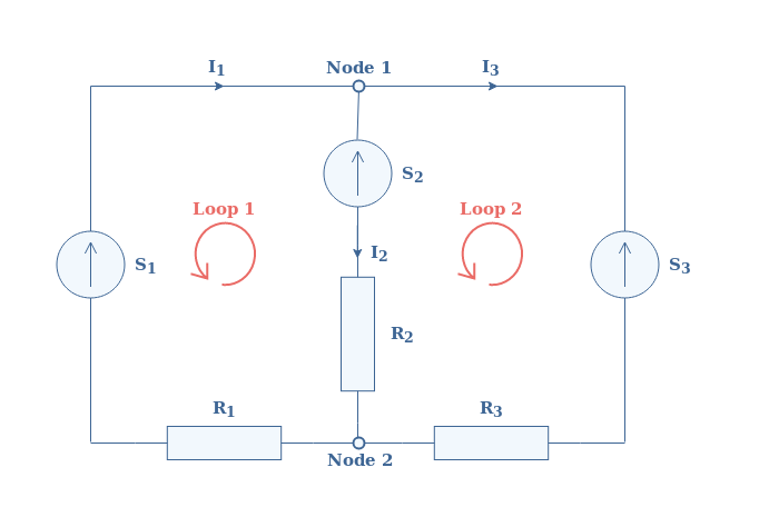
The sources are DC and ideal, meaning that they present no internal resistances. We take S₁=4 V, S₂=3 V, S₃= 10 V, and R₁=3 Ω, R₂=2 Ω, R₃=1 Ω.

From Kirchoff’s current law, we can write the following equalities for Nodes 1 and 2:

• Node 1: I₁=I₂+I₃
• Node 2: I₂+I₃=I₁ which is similar than the equation of Node 1

From Kirchoff’s voltage law, we write the equalities for Loops 1 and 2:

• Loop 1: S₁=S₂+R₂×I₂+R₁×I₁
• Loop 2: S₂+R₂×I₂=S₃+R₃×I₃

We can differently write these equations to obtain the following system of 3 equations with 3 unknown parameters I₁, I₂ and I₃:

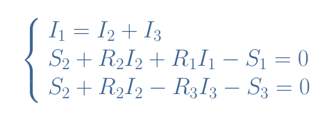
This system can be solved with the elimination method which consists of replacing I₁ by I₂+I₃ in the second line (L2) and eliminate the term I₃ by doing the addition R₃×L2+R₁×L3.

We find directly I₂=4.2 A, we can then find I₃ by replacing I₂ in L3 which gives I₃=1.4 A and finally we get I₁=I₂+I₃=5.6 A.

Limits of KCL

In the first section, we have seen the framework where KCL apply but there are also some other more subtle conditions that a circuit must respect. We briefly highlight in this section these further conditions for KCL to be valid.

The first condition is known as the quasistatic approximation and consists to say that the propagation time of the signal must be negligible compared to the period of the signal, this gives a condition on the dimensions of the circuit.

For example, consider an AC signal of 200 kHz (T=5 μs), if a receptor is located in the circuit at D=10 cm, the propagation time will be Δt=D/c=0.33 ns with c being the speed of light. In this case, Δt<<T, the quasistatic approximation is valid and the condition to apply KCL is respected.

However, if the receptor is located instead at D=1 km, the propagation time becomes Δt=3.3 μs and the inequality Δt<<T is not respected, therefore the approximation is not valid and KCL cannot be applied to the circuit.

This affirmation can be demonstrated with the Maxwell-Ampere equation in which the variating term can be eliminated when the quasistatic approximation is valid, the Kirchoff’s current law can then be demonstrated by using the Green-Ostrogradski theorem.

Another common condition to give validity to KCL consists to say that the variations of the magnetic flux across the loops of the circuit must be negligible. According to the induction law, variations of the magnetic flux create induced currents in the circuit and therefore induced voltages.

Conclusion

The KCL are fundamental laws of electronics that can be applied to electrical circuits constituted with loops and nodes. These topological definitions along with others are presented in the first section of the article that provides the framework in which the KCL are applied.

Kirchoff’s laws consist of a current and a voltage law that reflects the principle of conservation of energy in a circuit.

The current law accounts for the charge conservation, it states that the algebraic sum of currents in a node is equal to zero. The voltage law states that the algebraic sum of voltages in a loop is equal to zero.

It is presented in a further section that the use of both these laws can solve typical electronic problems by solving systems of linear equations.

Finally, we briefly present in the last section that some subtle conditions about the dimensions of the circuit and the existence of an external magnetic flux must be respected in order for the KCL to be valid.

Please follow and like us: