Nodal Voltage Analysis and Mesh Current Analysis

Introduction

As we have seen in the previous tutorial presenting the fundamental laws of circuit analysis, Kirchoff’s Circuit Laws (KCL) are a powerful and efficient tool to compute unknown voltages and currents in any circuit. However, KCL sometimes presents the inconvenience to be repetitive and is not the fastest way to analyze more complex circuits.

There are two methods based on KCL that simplify and make the analysis of circuits more efficient: the Nodal Voltage Analysis and the Mesh Current Analysis.

We separately present in this article both methods in two sections. In each section, a real example is given to illustrate how to perform these analyses.

Nodal Voltage Analysis

Presentation

The Nodal Voltage Analysis (NVA) is based on Kirchoff’s Current Law and is used to determine unknown voltages at the nodes of a circuit. It consists of a series of steps to follow, that are abstractly listed below:

1. Label the essential nodes of the circuit, essential nodes consist of nodes that are the junction between three or more branches.
2. Choose one of the nodes to be the reference of the circuit. In most cases, it is the bottom node.
3. Express the currents in the branches as a function of the voltages.
4. Write Kirchoff’s current law at each node other than the reference node.

Example

Consider the following electronic circuit presented in Figure 1 for which we will perform an NVA. For numerical applications, we take S₁=10 V and S₂=2 A; R₁=1 Ω, R₂=5 Ω, R₃=2 Ω, and R₄=10 Ω.

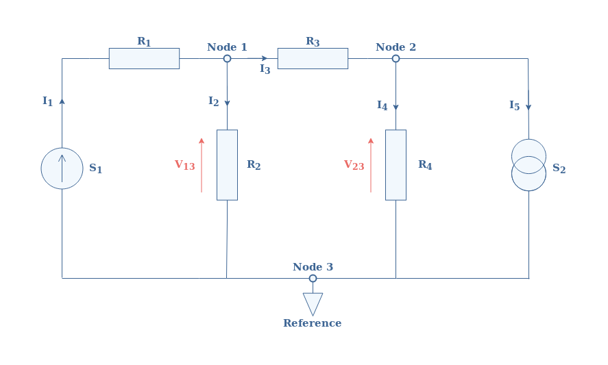
In this circuit, we already completed steps 1 and 2, the Node 3 has been chosen as the reference (ground) of the circuit, which is indicated with a grounding symbol.

According to step number 3, we can write each current I₁, I₂,…, I₅ as a function of V₁₂ and V₁₃, the currents are computed by applying Ohm’s law to each branch:

• I₁=(10-V₁₃)/R₁
• I₂=V₁₃/R₂
• I₃=(V₁₃-V₂₃)/R₃
• I₄=V₂₃/R₄
• I₅=-S₂=-2 A

According to step 4, we write the Kirchoff’s current law at nodes 1 and 2:

• Node 1: I₁-I₂-I₃=0 ⇒ [(10-V₁₃)/R₁]-[V₁₃/R₂]-[(V₁₃-V₂₃)/R₃]=0
• Node 2: I₃-I₄-I₅=0 ⇒ [(V₁₃-V₂₃)/R₃]-[V₂₃/R₄]+S₂=0

We obtain therefore a linear system of 2 equations with 2 unknown parameters that can be rewritten clearer by multiplying the lines with appropriate factors, arranging the terms and replacing the resistor and sources terms by their value:

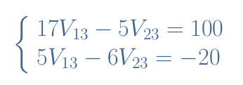
This system can be rewritten as a matrix equation:

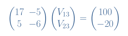
This type of equation can easily be solved by hand or using a computer program such as MatLab, the solution is V₁₃=9.1 V and V₂₃=10.1 V.

Since every current is a function of these values, we can compute and list them:

• I₁=(10-9.1)/1=0.9 A
• I₂=9.1/5=1.8 A
• I₃=(9.1-10.1)/2=-0.5 A
• I₄=10.1/10=1 A
• I₅=-2 A

Mesh Current Analysis

Presentation

Another powerful method that simplifies the KCL such as the Nodal Voltage Analysis is presented in this section and known as the Mesh Current Analysis (MCA). Instead of focusing the analysis around the nodes such as presented for the previous method, we label the currents circulating in each mesh of the circuit. A mesh simply consists of a loop with no other internal loops in it.

We list below the following steps to perform an MCA:

1. Attribute and label currents on each mesh of the circuit. Usually, we choose the clockwise direction for positive currents.
2. Apply Kirchoff’s voltage law (KVL) for every mesh in the same direction as the currents previously stated.
3. Solve the loop equations that appear with the KVL analysis.
4. Compute the required current or voltage in the circuit thanks to the mesh currents.

Example

Consider the following circuit illustrated in Figure 2 for which we will perform an MCA. The values of the different elements are given: S₁=12 V and S₂=6 V; R₁=15 Ω, R₂=2 Ω, and R₃=12 Ω.

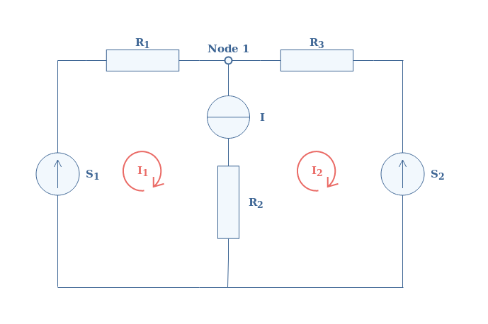
Step number one has already been done in the circuit where the mesh currents are labeled with the red loop symbols.

As step number 2 suggests, we apply KVL for each mesh of the circuit:

• Equation 1: -V₁+I₁×(R₁+R₂)-I₂×R₂=0
• Equation 2: V₂-I₁×R₂+I₂×(R₂+R₃)=0

In our case, both mesh currents I₁ and I₂ are present across the resistor R₂, in both equations we can see that the current across R₂ is considered as the algebraic sum of I₁ and I₂.

In the following, we replace the parameters by their value, first of all, we express I₁ as a function of I₂ thanks to the first equation:

• I₁=(12+2×I₂)/17

We substitute this term in Equation 2, which after redistributing the terms, leads to find I₂=-1/3 A. We put this value in the expression of I₁ to find I₁=2/3 A.

Finally, we can give the required current I to drive the circuit I=I₁-I₂=1 A.

Conclusion

We have presented in this tutorial two methods based on the Kirchoff’s Circuit Laws called the Nodal Voltage Analysis (NVA) and the Mesh Current Analysis (MCA). These methods are more efficient to analyze circuits because they lead to the solution faster than KCL by reducing the amount of mathematics involved.

Each analysis consists of a series of steps to perform, the methods are presented separately at the beginning of their respective section.

Examples are also given in order to show how to analyze resistive circuits with these two methods. We can note that for reactive circuits with inductors and capacitors, the NVA or MCA analysis leads to a differential equation or a system of differential equations to be solved.

Please follow and like us: