Parallel RLC Circuit Analysis

Introduction

The series behavior of the three elementary components of electronics has been detailed in our previous article Series RLC Circuit Analysis. In this tutorial, another association known as the parallel RLC circuit is presented.

In the first section, we present the elementary parallel RLC circuit and focus on its impedance.

The second section focuses on the AC behavior of the parallel RLC circuit. We highlight and explain the phenomenon of the resonance due to a parallel L//C configuration that explains some properties of parallel RLC circuits.

To conclude these two articles about RLC circuits, alternative configurations are presented in the last section.

Presentation

The parallel RLC circuit consists of a resistor, capacitor, and inductor which share the same voltage at their terminals:

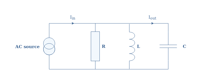
Since the voltage remains unchanged, the input and output for a parallel configuration are instead considered to be the current.

For a parallel configuration, the inverse of the total impedance (Z_RLC) is the sum of the inverse impedances of each component: 1/Z_RLC=1/Z_R+1/Z_L+1/Z_C. In other terms, the total admittance of the circuit is the sum of the admittances of each component.

This total admittance satisfies:

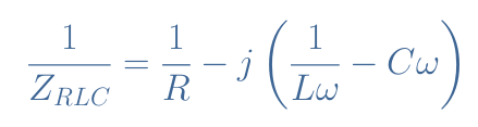
The total impedance is therefore given by Equation 1 after taking the norm of the admittance:

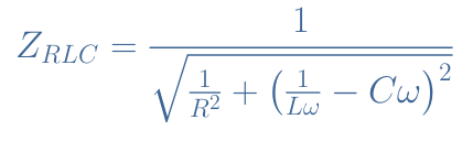
From Equation 1, it is clear that the impedance peaks for a certain value of ω when 1/Lω-Cω=0. This pulsation is called the resonance pulsation ω₀ (or resonance frequency f₀=ω₀/2π) and is given by ω₀=1/√(LC).

AC behavior

Fast analysis of the impedance can reveal the behavior of the parallel RLC circuit. Consider indeed the following values for the components of the parallel RLC circuit: R=56 kΩ, L=3 mH, and C=5 nF.

From these values, we can compute the resonance frequency of the system ω₀=2.6×10⁵ rad/s. The circuit is supplied by an AC source which amplitude is 5 A and frequency varies from DC to 4×10⁵ rad/S.

Figure 2 is a plot of the total impedance and output current as a function of the angular pulsation ω supplied to the circuit:

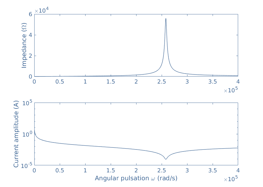
It is clearly evidenced by this figure that around the resonance frequency, the impedance of the circuit peaks, which leads to a decrease of the current output around this same frequency.

Let’s focus on what happens in the circuit and more precisely between the capacitor and inductor in order to understand this behavior. Consider, therefore, to begin with, an L//C configuration in which the capacitor is initially charged. The following Figure shows the steps involved in a cycle called resonance:

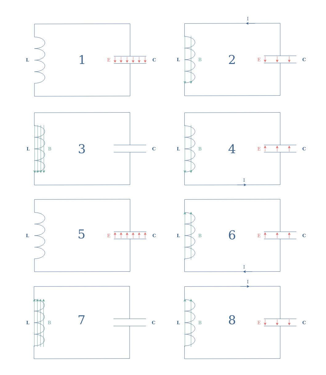
Many things must be commented in Figure 3. First of all, the red and green arrows represent respectively the electric field across the capacitor and the magnetic field across the inductor. The arrows indicate the direction of the fields, a fully charged component is represented with many arrows while a discharged component has none.

The numbers represent the steps of the cycle, the next step after number 8 is step number 1. As highlighted in this series of figures, the resonance phenomenon is due to mutual charges and discharges occurring between the capacitor and the inductor. The speed at which this cycle evolves is given by the resonance frequency f₀=1/(2π√(LC)).

In real circuits, this cycle is of course not perpetual as internal resistors dissipate energy by Joule’s heating. However, an AC source can force the circuit to maintain this exchange of current between the inductor and capacitor.

Specifically, when ω_source=ω₀, the exchange of energy is maximum and all the current is flowing in between these two components and none in the mainline across a resistance (see Figure 4). Another way to understand that is through the concept of reactance. We remind that the reactances of a capacitor (X_C) and an inductor (X_L) are given by:

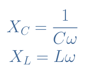
From the definition of ω₀, it comes that X_C(ω₀)=X_L(ω₀). The currents across the components are therefore equaled but of opposite directions due to the phase-shifts of +90° in the inductor and –90° in the capacitor leading to a phase difference of 180°. This phenomenon can be seen in steps 2 and 4 or steps 6 and 8 in Figure 3.

When working around ω₀, this configuration is commonly known as a rejector circuit. We detail this more in the following section where we show that an L//C circuit can be connected in series with a resistor to create a band-stop filter.

Alternative configurations

Band-stop filter

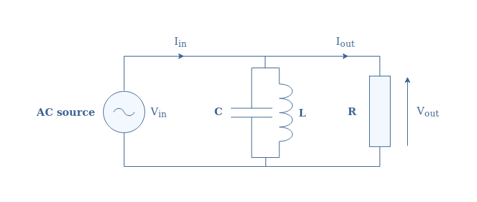
One possible interesting configuration that mixes both a parallel and series design is a parallel LC filter in series with an output load, we will call this circuit (L//C)-R in the following. A representation of this architecture is given in Figure 4 below:

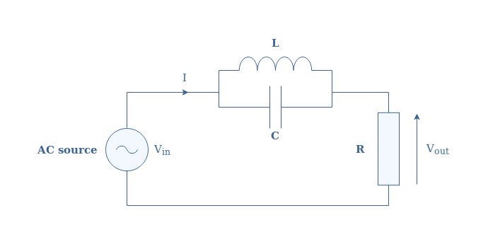
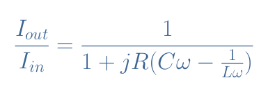
If we call Z_L//C the impedance of the parallel LC configuration, we can write that V_in=V_out+Z_L//C×I. Knowing that I=V_out/R and by factorizing the expression by V_out, we can write after a few steps the transfer function of the (L//C)-R circuit:

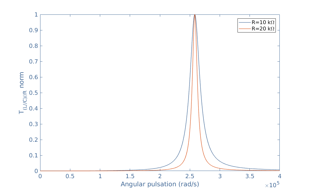
We consider L=3 mH, C=5 nF, and R=10 kΩ and 20 kΩ. It becomes clear after plotting this transfer function that the (L//C)-R circuit act as a band-stop filter around the same frequency ω₀ as for the elementary parallel RLC circuit_:

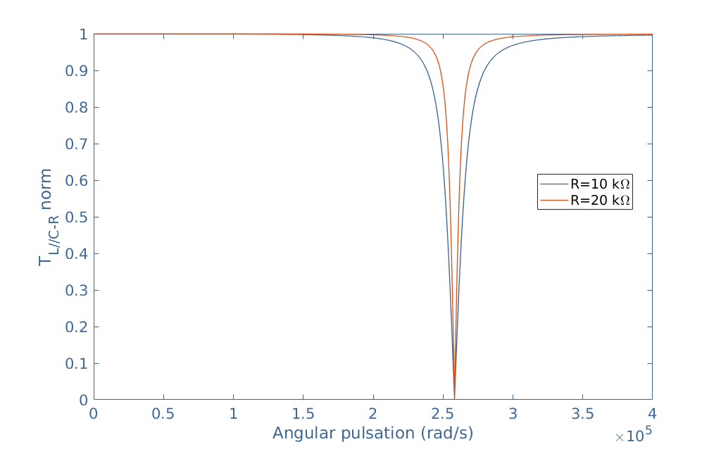
Figure 5 also highlights the fact that the bandwidth Δω of this band-stop filter becomes narrower when the resistance increases, which is in contradiction with the definition of the quality factor given in the series RLC article Q_series=(1/R)√(L/C)=ω₀/Δω.

In fact, this definition is not valid for parallel circuits, the formula for a parallel configuration becomes Q_parallel=1/Q_series=R√(C/L), which explains the behavior in Figure 4 previously pinpointed.

Band-pass filter

An interesting concept called duality enables us to directly find the behavior of a new circuit from the knowledge of another. It is deduced from the fact that the equations applying to the current or voltage to a certain configuration can be applied to the dual quantity of the dual configuration.

Let’s be a little clearer and consider again the band-stop filter example detailed above. We call this configuration (L//C)-R since a parallel (//) LC circuit is in series (-) with a resistance R. We have seen that this circuit act as a band-stop filter for the voltage.

The dual of this circuit is a (L//R)//R circuit illustrated in Figure 6:

The duality concept tells us that this dual circuit acts as the dual of a band-stop filter, which is a band-pass filter. To verify this affirmation, we can start by writing that I_in=I_out+Y_L//C×V_out which is the same equation shown in the previous section but applied for the current, as stated by the duality concept. Y_L//C is the admittance of the configuration L//C and equals 1/Z_L//C.

Knowing that V_out=R×I_out and by factorizing the expression with I_out, it comes:

We can see that Equation 3 is very similar to Equation 2 but the imaginary term is inversed which leads to the band-pass filter behavior. We can consider again the same values L=3 mH, C=5 nF, and R=10 kΩ and 20 kΩ and plot this transfer function in order to conclude this section and confirm about the band-pass filter:

Conclusion

The behavior of a parallel RLC circuit is quite different than the series configuration. This is due to the phenomenon of reciprocal exchange of energy of the L//C circuit called resonance.

This phenomenon is due to the mutual discharges/charges occurring between an interconnected inductor and capacitor. The impedance of such a circuit theoretically tends to an infinite value at a particular pulsation ω₀ called the resonance pulsation (or resonance frequency for f₀). In real circuits, this impedance peaks due to internal resistive behaviors.

We have seen in the last section, that integrated in series with an output load, a band-stop filter can be made. Connected in parallel, however, leads to the opposite filter: a band-pass filter.

Please follow and like us: