The Fourier Analysis – Fourier Series Method

Introduction

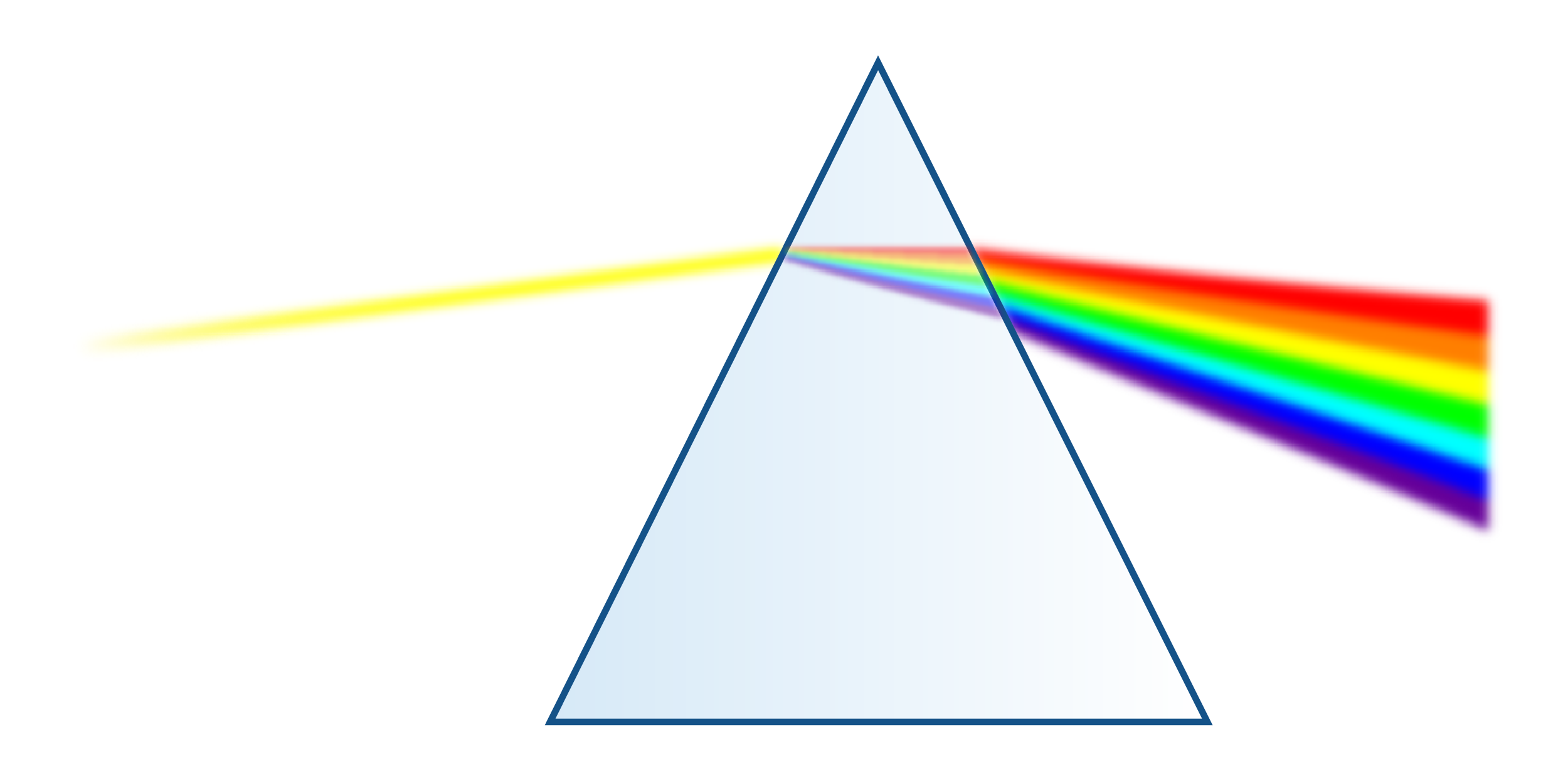
This subject was first assumed by Isaac Newton about 400 years ago. Newton showed that white light is composed of other colors. He called the color components of white light as “spectre”, from which we get the word spectrum. Figure 1 shows how a light beam is dispersed to some component colors i.e., waves with different frequencies from red (the lowest frequency of visible light) to violet (the highest frequency), after passing through a prism.

Then, Jean Baptiste Joseph Fourier (1768-1830), a French mathematical physicist, discovered that any periodic waveform can be represented as a sum of an infinite number of weighted sinusoids, i.e., sine and cosine waves. Fourier’s theory states that any periodic function can be synthesized using these sinusoidal waves. Generally, using more sinusoidal waves produces a better result. This sinusoid summation concept is called the Fourier series. Fourier Series deal with functions that are periodic over a finite time interval. These arbitrary functions are assumed to repeat outside this interval.

The basic building blocks of Fourier analysis come from a set of harmonic sinusoids, called the basis set. This basis contains an infinite number of periodic sinusoids of different frequencies known as harmonics. Each individual wave is named an element of the basis.

The process of decomposing an arbitrary periodic signal into a set of basic waves is termed Analysis. We can re-create the periodic signal by putting together (adding) some waves from the basis set. This process is called Synthesis.

Square wave analysis in the time domain

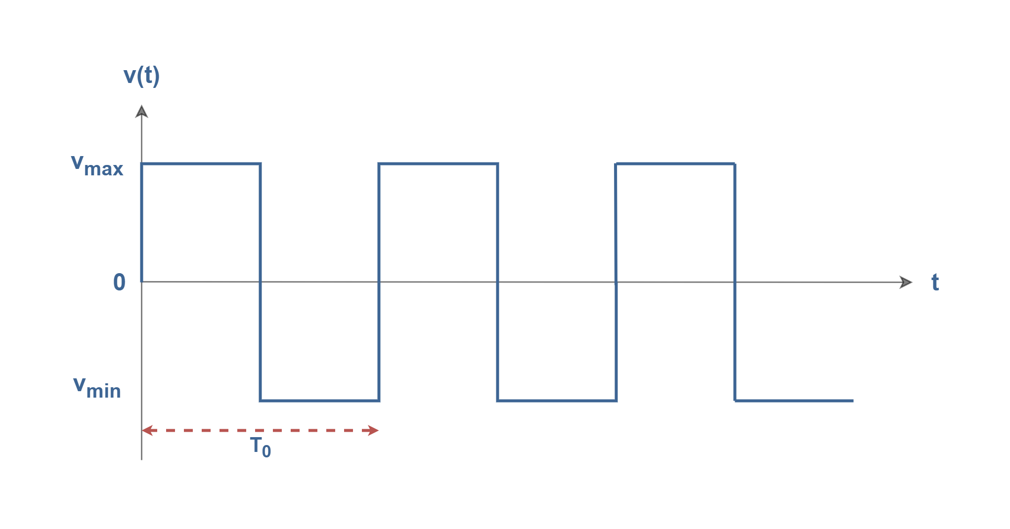
It is advantageous to examine the construction of a square wave as an example. The square waves are very useful in signal processing and data transmission. It is possible to create them by just adding a set of sinusoids. Figure 2 shows a pure square wave with a rectangular-shaped waveform in the time domain with a frequency of f₀ (= 1/ T₀) and with the maximum amplitude of V_max.

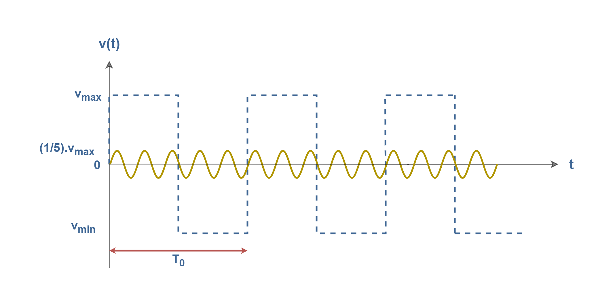
In Figures 3-1 to 3-5, we have created a square wave by adding together only a few harmonic sinusoids, i.e., the synthesis procedure. In Figures 3-1, we have only one sine wave with the fundamental frequency of f₀ (= 1/ T₀) and with the maximum amplitude of V_max.

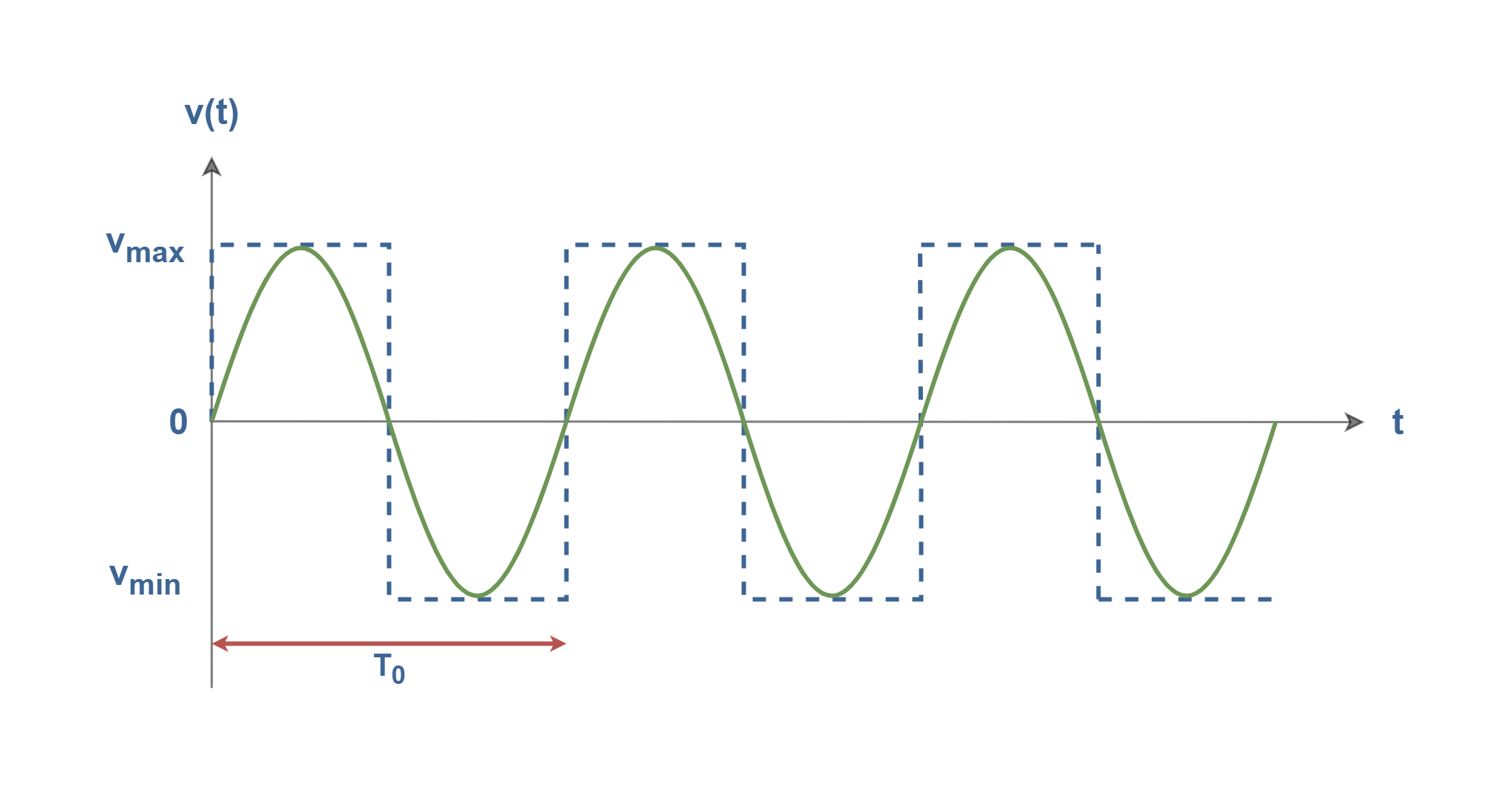
In Figures 3-2, we have the second sine wave with a frequency three times the fundamental (3f₀) and with the maximum amplitude of one-third of the original signal (V_max /3).

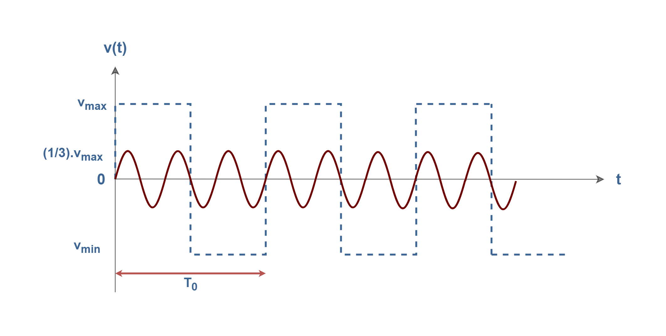
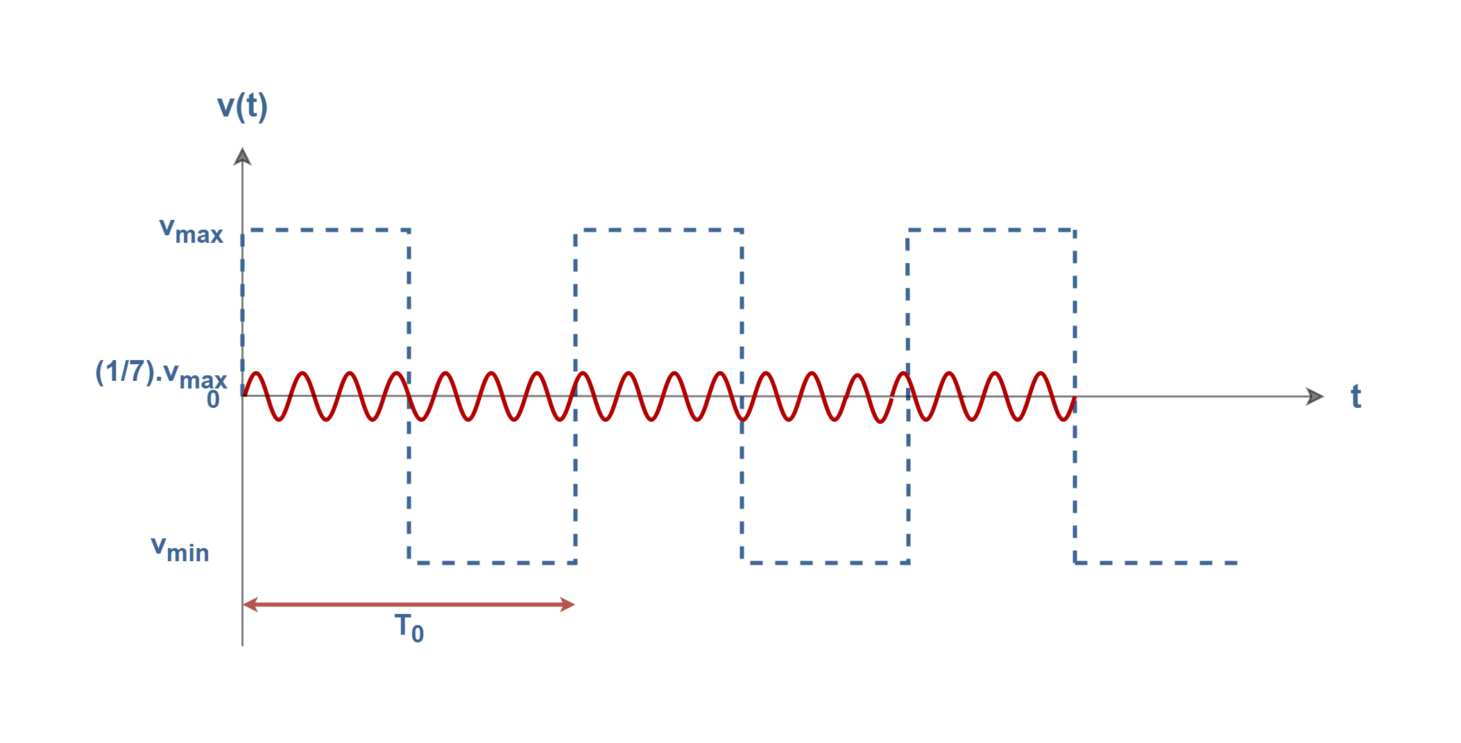
In Figures 3-3, there is the third sine wave with a frequency of five times the fundamental (5f₀) and with the maximum amplitude of one-fifth of the original signal (V_max /5).

Figures 3-4 show the forth sine wave with a frequency of seven times the fundamental (7f₀) and with the maximum amplitude of one-seventh of the original signal (V_max /7).

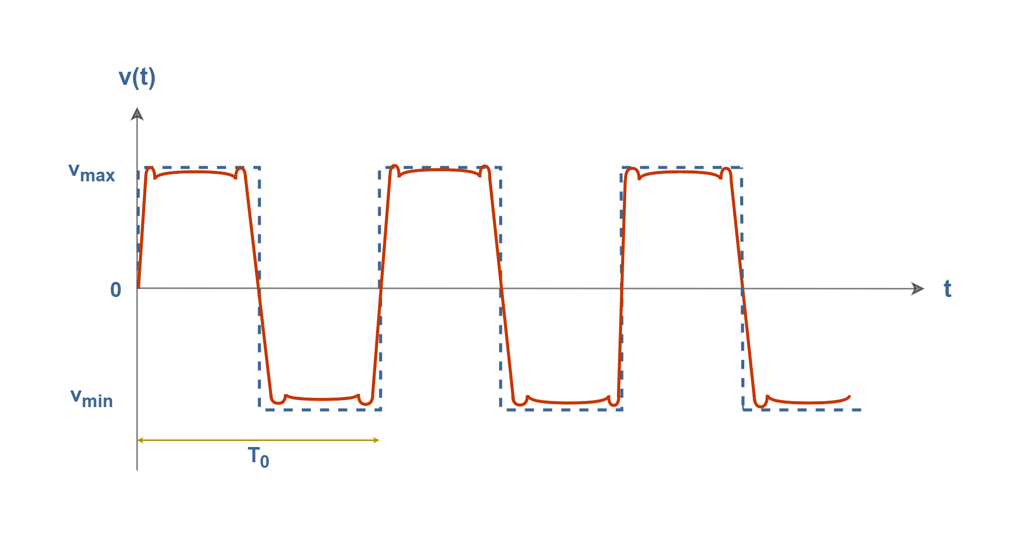
Finally, we add all of their amplitudes in each corresponding instance of time and the resultant waveform is shown in Figure 3-5.

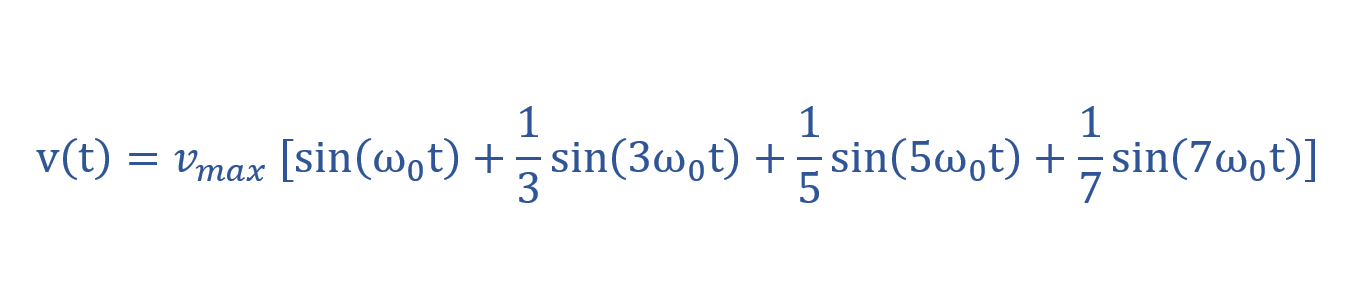
Hence, the steps that we took to make or synthesize a square wave by summing odd harmonics with different amplitudes can be explained in a simple mathematical model in Equation 1. This can be shown as a simple Fourier series.

Therefore, after analysis of the periodic signal into sinusoidal waves, the original time-domain signal is able to be reconstructed by adding together all the sinusoidal signals at every corresponding instance of time, i.e. the original signal is obtained from the superposition of component waves. This is the basic idea of the Fourier analysis method.

The more sinusoids we add to the summation, the better the wave looks, with the wiggles getting smaller. Hence, the Fourier series represents an estimate of the true representation, the accuracy of which depends on the number of terms used. Although, this form of harmonic representation may not result in a perfect reconstruction of the original signal.

Square-wave analysis in the Frequency domain

In the spectrum, the amplitude of each of the frequency components is identified. The spectrum of the signal shown in Figure 3-5 is composed of just four frequencies and can be drawn as illustrated in Figure 4.

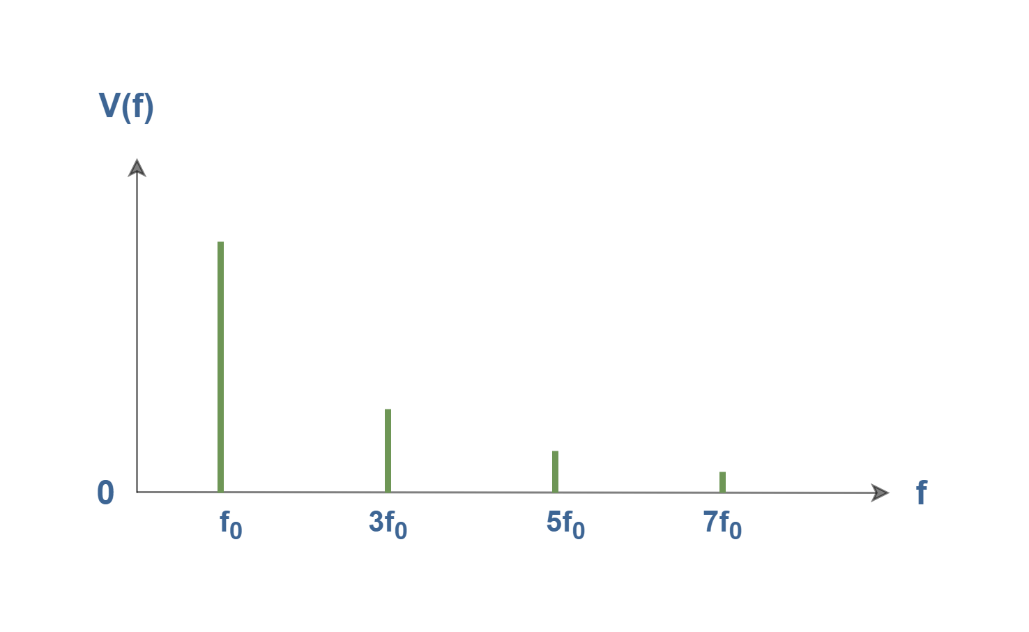
Basically, sine waves exist only at one frequency. The bandwidth of a single sine wave is zero. It produces a single vertical line on a spectrum analyzer. The x-axis in Figure 4 represents the component frequencies of the signal, whereas the y-axis is the amplitude of those frequencies. This is called a one-sided line spectrum.

The first and lowest frequency is called the fundamental frequency, f₀. Each harmonic frequency is an integer multiple of the fundamental. Each nth wave has a frequency that is equal to n times the fundamental frequency i.e., f_n = n.f₀ , where n is any arbitrary integer; 0, 1, 2, . . . ,∞. The frequency of the first harmonic and the fundamental frequency are the same (n = 1). The wave for n = 2 is called the second harmonic and so on for higher values of the index n.

The wave obtained for (n = 0) is called the DC component. In the above-mentioned signal of v(t), the DC component is zero.

The Fourier Series Method

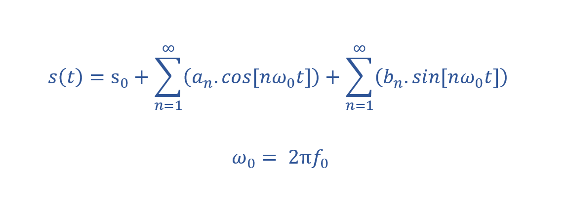
Assume that s(t) is given as an arbitrary periodic signal of period T₀. The Fourier series says that the signal s(t) is equivalent to a summation of some weighted sinusoids (harmonics). Equation 2 states a compact Fourier series formula containing the sum of trigonometric functions.

The coefficients s₀, a_n, and b_n are called the Fourier Series Coefficients. The process of Fourier analysis consists of computing these three types of coefficients, given an arbitrary periodic function, s(t). The constant s₀ is a DC offset and the coefficient a_n represents the coefficient of the n-th cosine wave and b_n of the n-th sine wave.

Equation 3 shows a simple method for computing the first coefficient s₀:

The result of the integration of the target signal s(t) over one period, normalized by the period, is equal to the 0-th coefficient. Therefore, the DC coefficient s₀ equals to the area under the given signal waveform in one period i.e., the mean power of the signal.

We can also write Equation 4 for computing a_n, the coefficients of cosine elements:

The coefficient a_n is computed by taking the integral of target signal s(t) multiplied with a cosine wave of n-th harmonic frequency over one period T₀. The result of the integration is then multiplied (or normalized) by 2/T₀ to obtain the coefficient for that particular harmonic. If we do this calculation n times, we get n independent a_n coefficients.

The process of computing the coefficients of the sine elements, b_n, is exactly similar. We can multiply the target signal s(t) sequentially by a sine wave of frequency, nω₀. Equation 5 shows the method:

Hence, the coefficient b_n can be calculated by multiplying s(t) by the n-th harmonic and integrating the expression.

Essentially, our assumption was based on periodic signals and our elements of the basis set were supposed to be eternal sinusoids. But, it is worth mentioning that obviously, no real signal goes on forever. Although, these equations could be a reasonable model for a sinusoidal waveform that lasts a long time compared to the period.

Coefficients make the spectrum

In the above-mentioned equations, the signal s(t) is expressed in the time domain. But, coefficients a_n and b_n (and especially the absolute values of coefficients |a_n| and |b_n|) can represent the amplitude spectrum of the signal s(t) as a function of frequency.

As a general example, we can consider an arbitrary periodic signal f(t) which is expressed in Equation 6:

The time-domain representation of the signal is shown in Figure 5:

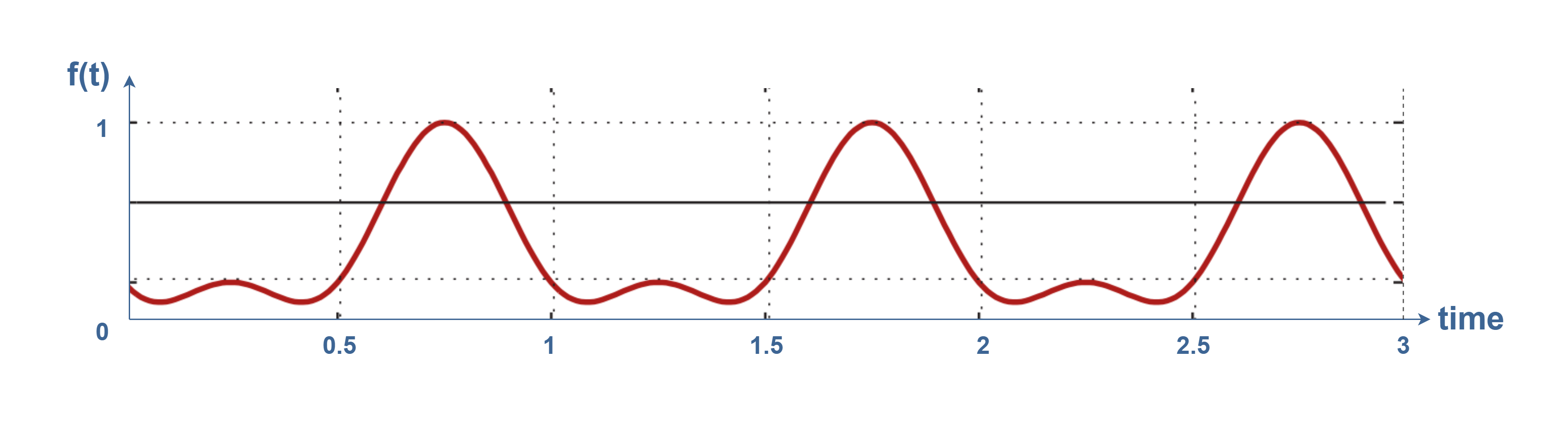
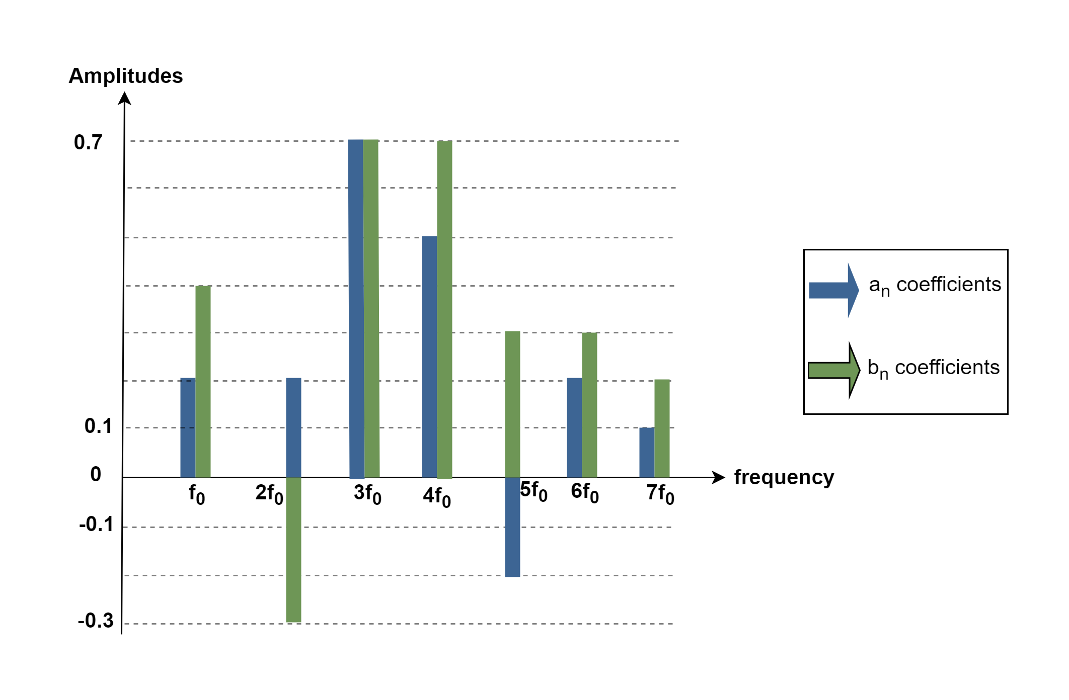
If we apply Equations 3, 4, and 5 on this function to find its Fourier series coefficients, we will find a DC coefficient and some non-zero sine (b_n) and cosine (a_n) factors. Assume that the trigonometric coefficients are calculated as values in Table 1:

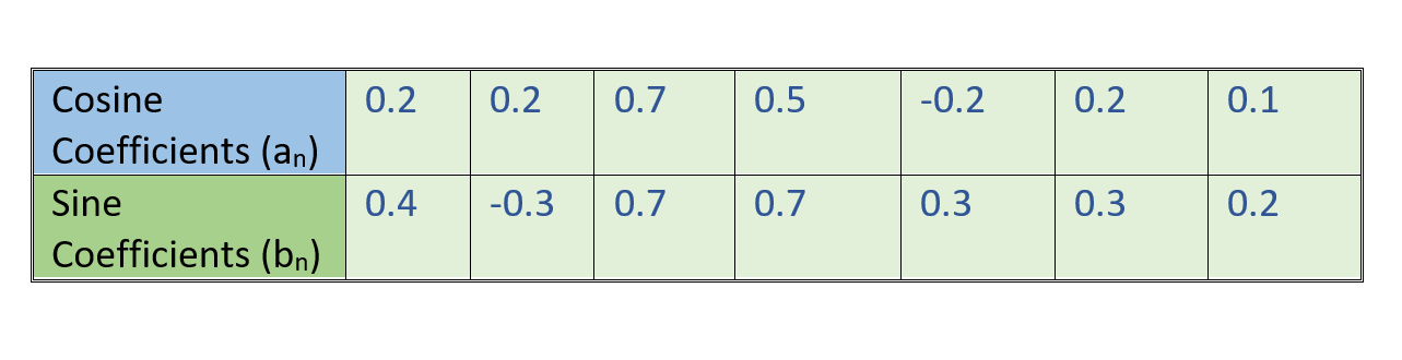
Figure 6 shows the coefficient values which are plotted as amplitudes in the frequency domain.

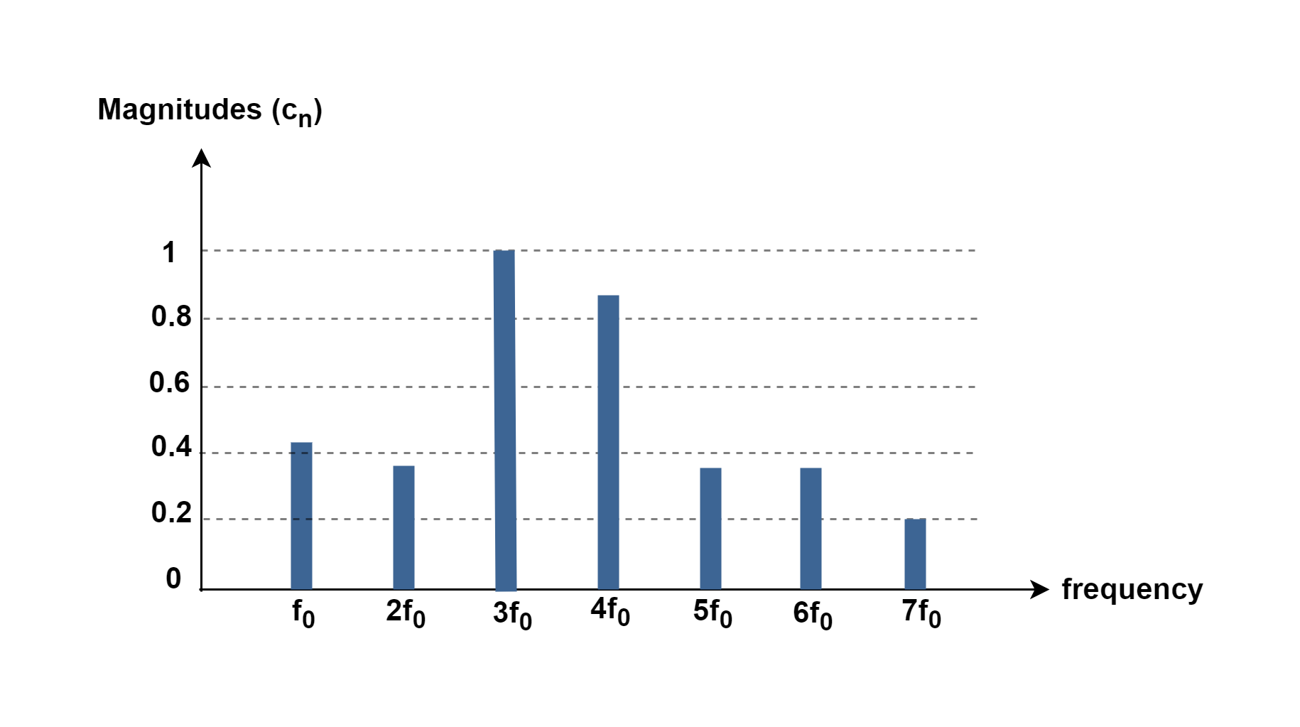
For better understanding and interpretation, a spectrum is supposed to have just one number for each frequency. So, it is better to combine the above-mentioned sine and cosine coefficients into two real-world quantities, called magnitude and phase.

As sine and cosine functions are orthogonal to each other (because of 90 degrees phase shift), and have the same frequency, therefore, we can compute their summation as 2 vectors. This calculation can be done by the root-sum-square (RSS) method for the two coefficients. The magnitude quantity, c_n, is one number for each frequency and is computed by the expression in Equation 7:

While in some cases the value of amplitude can be negative, the magnitude is always positive. The effect of the sign of the amplitude is now seen in a term called phase, which we calculate in Equation 8.

The range of arctan (x) is from −π/2 to +π/2, so it must cover the full phase values.

Figures 7 and 8 show these two quantities on a pair of plots, one for the magnitude and the other for the phase term, both plotted as a function of the harmonic frequencies.

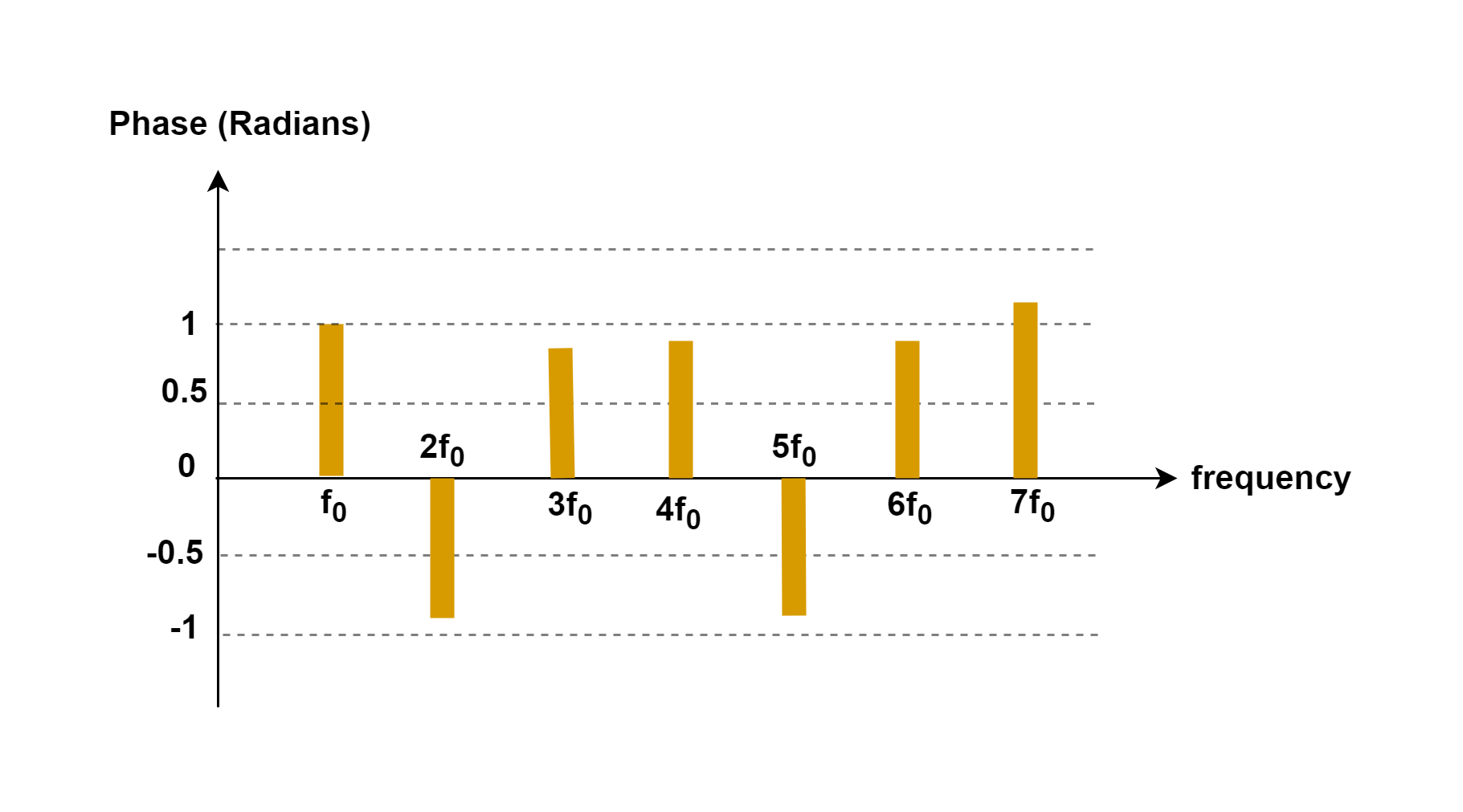
Normally, the magnitude spectrum is the preferred form in industry rather than amplitude. Its companion, the phase spectrum, usually does not offer practical information and for this reason, it can be ignored most of the time.

Conclusion

Describing continuous signals as a superposition of waves is one of the most useful concepts in many branches of science like electronics, physics, acoustics, optics, and so on.

Based on mathematical Fourier analysis, many types of periodic signals can be decomposed into a combination of sine waves. Also, it is possible to create any periodic signal by the summation of a particular set of harmonic sinusoids.

The result of the synthesis method in Figure 3-5 looks good but it is not a perfect square-wave shape. Because it is not possible to synthesize ideal periodic functions that have discontinuities in their waveforms. Discontinuities are events that occur in zero time. An ideal square wave changes from a maximum positive value to a maximum negative value in zero time. There is no such thing in the real world.

One of the main features of the Fourier Analysis rules is to find the spectrum of different periodic waveforms such as the Saw-tooth wave and so on. Practitioners often need to understand of the basis of spectral estimation of different signals.

Summary

• The Fourier analysis technique was invented by Joseph Fourier in the early 19th century.
• The term periodic signal is usually applied to periodically varying voltages, currents, or electromagnetic fields. The Fourier series concept is a powerful mathematical tool for better analyzing of time-periodic signals.
• The sines and cosines, those having a fundamental frequency and all the corresponding harmonics, are said to form a basis for all periodic waveforms. Each of the sine or cosine waveforms is an element of the basis. This means that not only can sines and cosines be combined to construct any complicated periodic waveform, but also any complicated periodic waveform can be broken down into the sum of sines and cosines.
• The Fourier analysis process consists of finding the series coefficients.
• If a periodic signal s(t) of period ‘T’ is a real function of time, then, it can be decomposed into a summation including some components:
  • – A term s₀ representing the average value or DC component of the signal;
  • – A sinusoidal term of frequency f (= 1/T) called the fundamental or 1^st harmonic term;
  • – A series of sinusoidal terms with frequencies that are multiples of ‘f’ called harmonics.
• By using the Fourier analysis method, it is possible to change the representing domain of the signal from time to frequency.
• The more terms we add, the closer we get to what we are trying to achieve.
• There is no such thing as an ideal square wave in any physical or electrical system.

Please follow and like us: