Thevenin’s Theorem

Introduction

In this tutorial, we present a powerful method that can simplify through some transformation steps, complex circuits into elementary circuits and this method is commonly known as Thevenin’s theorem.

Originally, it was the German physicist Hermann von Helmholtz who first demonstrated the theorem in 1853, but history kept the name of the French engineer Leon Thevenin, who in 1883, unawarely of the work of Helmholtz, proposed a more elegant method to prove the theorem.

We will illustrate this statement in the first section where we also define the bold terms of the theorem. In the second section, we present the method to follow in detail, in order to apply Thevenin’s theorem to a circuit.

Finally, some Thevenin transformations are fully depicted in the last section with real circuits taken as examples.

Presentation and definitions

As previously mentioned, Thevenin’s theorem can only be applied to linear electrical circuits (LEC). The internal structure of LEC consist of interconnected ideal sources and resistors. Reactive components such as capacitors and inductors must be excluded since their voltage/current characteristics are not described by a linear formula.

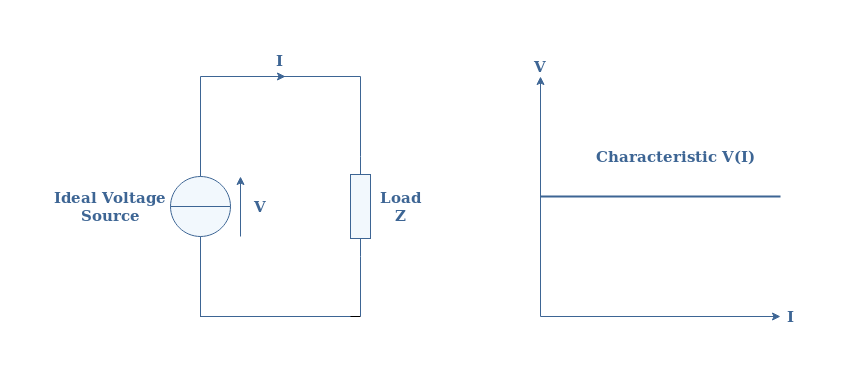
An ideal voltage source consists of a generator that delivers a constant value of voltage regardless of the current flowing in the circuit. This means that the same ideal source will always deliver the same voltage V_s for any circuit connected at its terminals. This property ensures that the voltage/current characteristic of an ideal voltage source is constant and therefore is linear.

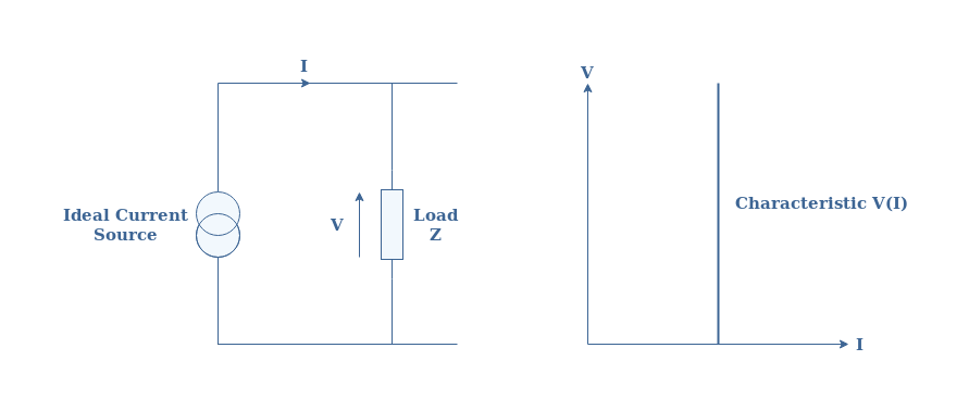
Ideal current sources can also be found in LEC and consist of generators that provide a constant value of current regardless of the voltage at their terminals. A representation of an ideal current source along with its and voltage/current characteristic is proposed in Figure 2 below:

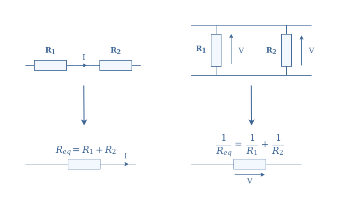
An equivalent resistor R_eq is simply a concept that represents the association of a set of interconnected resistors (R₁, R₂,…) into a single component. The association of resistors is dictated by two rules:

1. If the resistors share the same current (in series), the equivalent resistance is the sum of the resistors.
2. If the resistors share the same voltage (in parallel), the inverse of the equivalent resistance is the sum of the inverses of the resistors.

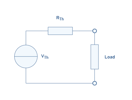
Now that these various definitions have been detailed, we can illustrate Thevenin’s theorem with the following Figure 4:

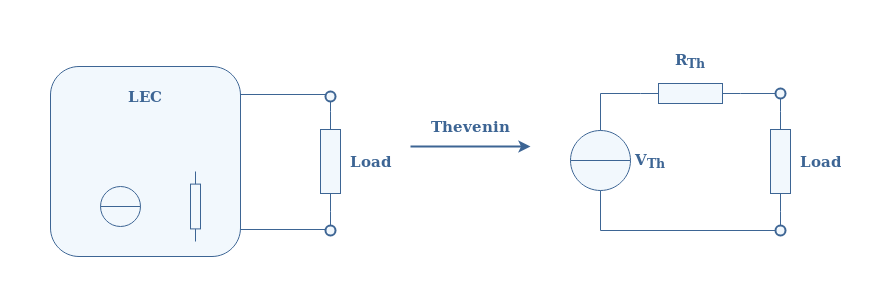
The simpler circuit obtained from the Thevenin transformation is known as the Thevenin model. The equivalent source and resistance are labeled with the subscript Th as a reference to the name of the theorem.

In the next section, we give the abstract method in order to determine this model from any LEC.

Thevenin model determination

The goal of this section is to present how the Thevenin parameters V_Th and R_Th are determined.

Thevenin’s voltage V_Th is the voltage between the terminals of the LEC when the load is disconnected and it is also known as the open-circuit voltage.

Similarly, Thevenin’s resistance R_Th is the resistance at the terminals of the circuit when the load is disconnected and all the circuit’s sources are disabled, the voltage sources are replaced with short-circuits and the current sources with open-circuits.

We propose therefore a series of steps to follow in order to determine the Thevenin model of any LEC:

1. Remove the load at the terminals of the LEC
2. Compute the voltage of the open-circuit
3. Replace any voltage sources with short-circuits and the current-sources with open-circuits
4. Compute the equivalent resistance
5. Reconnect the load and draw the Thevenin model thanks to the knowledge of V_Th and R_Th

In the following section, we illustrate this method by determining the Thevenin model of some LEC examples with increased architecture complexity.

Thevenin’s model of some LEC

Single voltage source

For the first example, we consider a basic LEC composed of only one voltage source and two resistors in a parallel configuration:

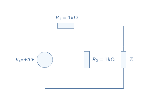
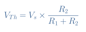
In order to determine Thevenin’s model, first of all, we proceed to steps number 1 and 2 explained in the previous section. When disconnecting the load Z from the circuit, we compute the voltage at the terminals of the LEC, that is to say across the resistor R₂, by applying the voltage divider method:

After replacing the parameters by their values, we obtain V_Th=2.5 V.

We consider now the circuit by replacing the voltage source by a wire. The equivalent Thevenin resistance is the parallel association of the resistors R₁ and R₂:

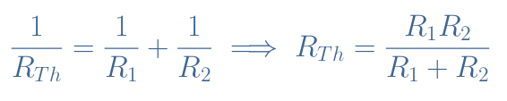
The numerical application gives R_Th=500 Ω.

The circuit presented in Figure 5 can, therefore, be simplified by the equivalent Thevenin’s model presented in Figure 6:

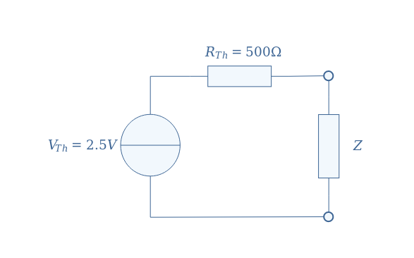
The voltage and current across any load Z are now much easier and faster to compute. As an example, if Z=100 Ω, we can use again the voltage divider formula to find V_Z=0.4 V. The current is obtained by applying Ohm’s law to the resistance Z: I=V_Z/Z=4 mA.

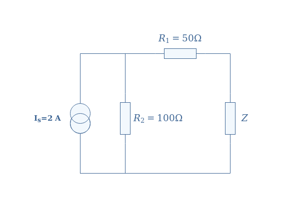
Single current source

For the second example, we consider a similar circuit than in Figure 5, but replacing the voltage source by an ideal current source and rearranging the resistors:

First of all, we disconnect the load Z from the circuit in order to determine V_Th:

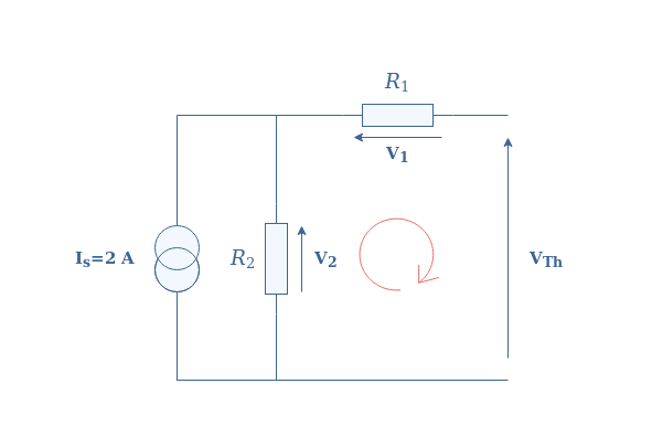
When applying Kirchoff’s Voltage Law in the loop highlighted with the red symbol, we find V_Th=V₂-V₁. However, since the circuit is opened, no current is observed across R₁ and therefore V_Th=V₂. The current flowing in R₂ is thus equal to the current source, we finally apply Ohm’s law to R₂ in order to find V_Th=100×2=200 V.

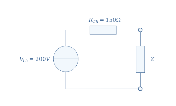
Thevenin’s resistance R_Th is found by replacing the current source by an open circuit, the equivalent resistor is determined by the series association of R₁ and R₂: R_Th=R₁+R₂=150 Ω.

Figure 8 below illustrates the Thevenin model of the circuit presented in Figure 7:

Multi-current/voltage sources

For this last example, we propose a more complex circuit that includes both current and voltage sources:

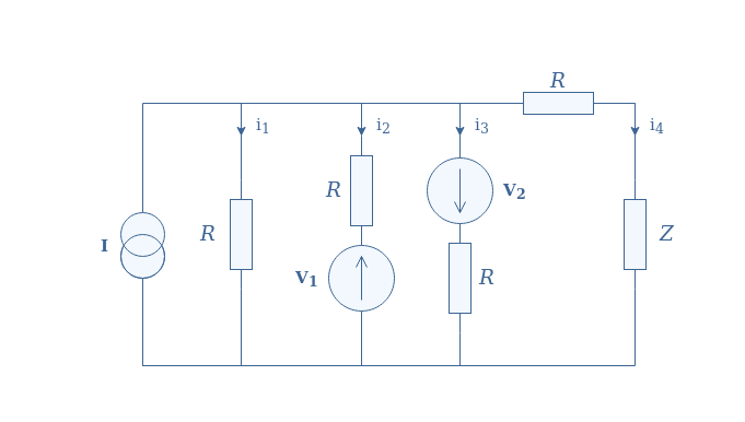
We disconnect the load in order to determine the voltage V_Th. It comes automatically that i₄=0 since the circuit becomes open. Kirchoff’s current law affirms that I=i₁+i₂+i₃, moreover, we can assert thanks to Kirchoff’s voltage law that:

• i₁=i₂+V₁/R
• i₁=i₃-V₂/R

After rearranging these three equations, we can isolate i₁=(I+V₁/R-V₂/R)/3. Thevenin’s voltage is simply given by R×i₁, therefore, V_Th=(RI+V₁-V₂)/3.

We replace the current source by an open circuit and shorten the voltage sources in order to determine R_Th:

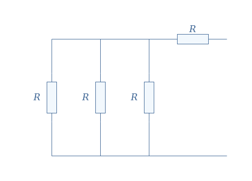
The equivalent resistance is given by the parallel association of 3 resistors in series with R, which leads to R_Th=R+R/3=4R/3.

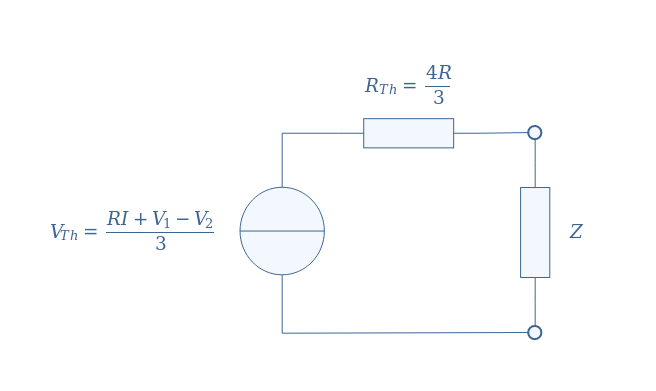
Thevenin’s model of Figure 9 is finally given by:

Conclusion

“Any linear electrical circuit is equivalent to an ideal voltage source in series with an equivalent resistor.” This sentence, known as Thevenin’s theorem, was the focus of this article.

In the first section, we define the bold terms which give the framework where the theorem can be applied. A linear electrical circuit (LEC) is an interconnection of ideal sources and resistors. Ideal sources are further defined as sources with a perfectly flat voltage/current characteristic. An equivalent resistor is simply a concept that allows us to regroup a set of interconnected resistors into a single component.

In a short second section, we abstractly present how to determine the Thevenin model of any LEC by following a series of steps.

The third section illustrates, with real examples, how to transform a LEC into its equivalent Thevenin’s model. First, we clarify how to proceed for circuits containing either voltage or current sources. Finally, we demonstrate how to perform the transformation with a more complex LEC containing both sources and more resistors.

It becomes especially clear with the last example that Thevenin’s model is a powerful tool to transform complex linear circuits into elementary circuits containing only one source and a resistor.

Please follow and like us: