Two-Port Parameters and Transformations

Introduction

A linear circuit is one whose output signal is linearly proportional to its input signal. As a simple case, it is possible to model the network at only two terminals as shown in Figure 1. Here, only V₁ and I₁ as the voltage and the current internal to the circuit, need to be described. A pair of terminals through which a current may enter or leave a network is known as a port. As shown in Figure 1, the current I₁ which enters one terminal ‘a’, equals the current leaving the other terminal ‘b’. Two-terminal devices or elements (such as resistors, capacitors, and inductors) can be characterized as one-port networks.

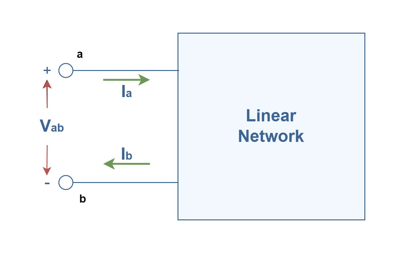
To establish a mathematical model for the network at the defined port, two further restrictions should be considered: (1) all external connections to the circuit, such as sources and impedances, are made at the port and (2) the network can have internal dependent sources, but not independent sources. Then, with the logical assumption of (I_a = I_b = I), we can rewrite Ohm’s law for this port as shown in Equation 1:

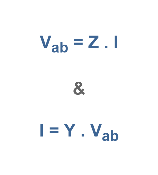
where Z is the impedance and Y is the admittance of the network at the port. In a mathematical model, the various terms that relate the voltage and the current are called parameters. Z and Y are parameters which can be in the form of Laplace transforms [Z(s) and Y(s)], sinusoidal steady-state functions [Z(jω) and Y(jω)], or simply constant resistive terms.

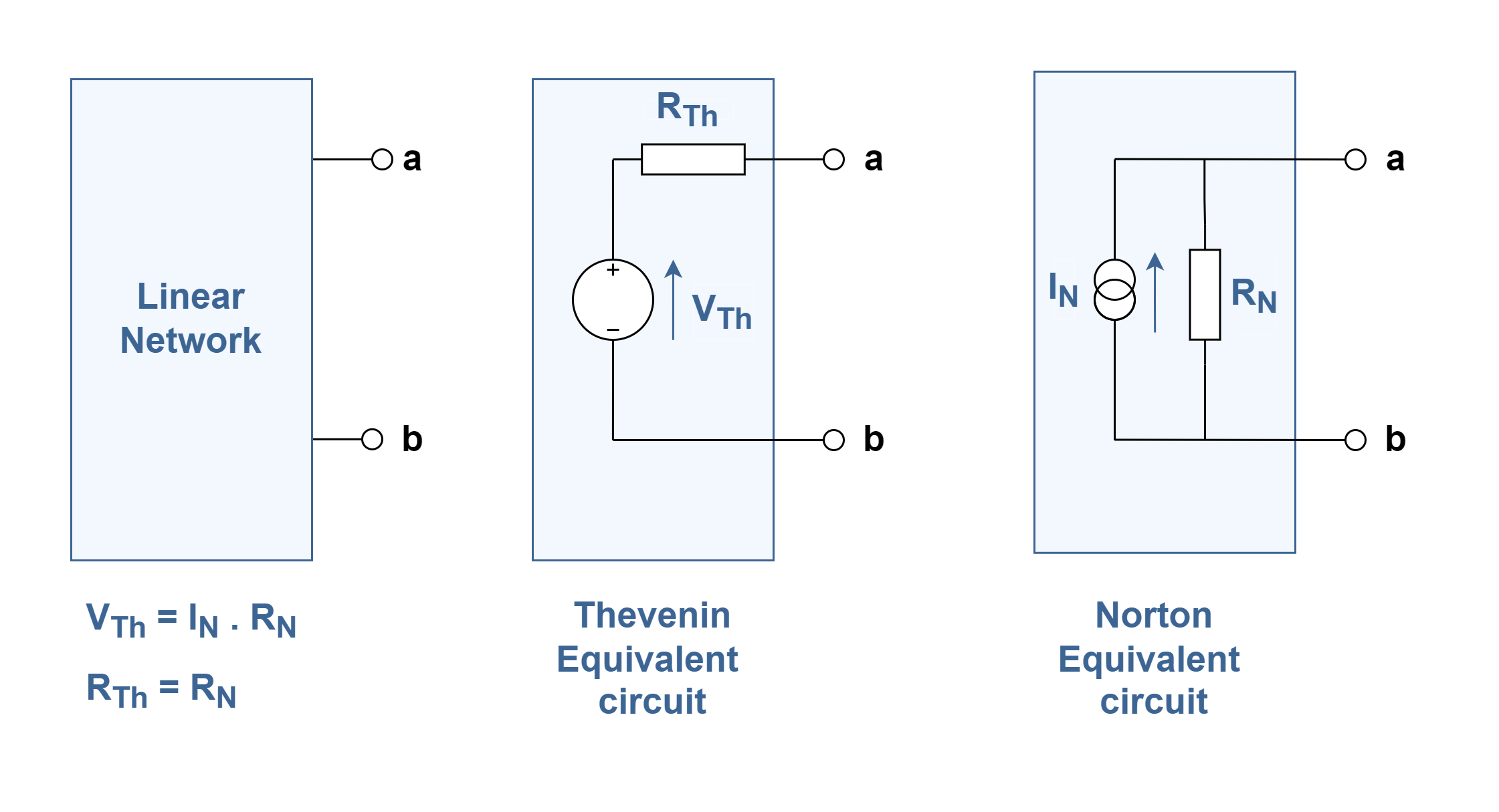
Generally, to analyze a linear electric circuit, Thévenin’s and Norton’s theorems can be used to produce a simplified behavior model of an electric/electronic network as viewed from the selected terminals. These theorems provide techniques by which the real network is replaced by an equivalent circuit. Figure 2 reviews these theorems. You can also find details about the theorems in the links attached.

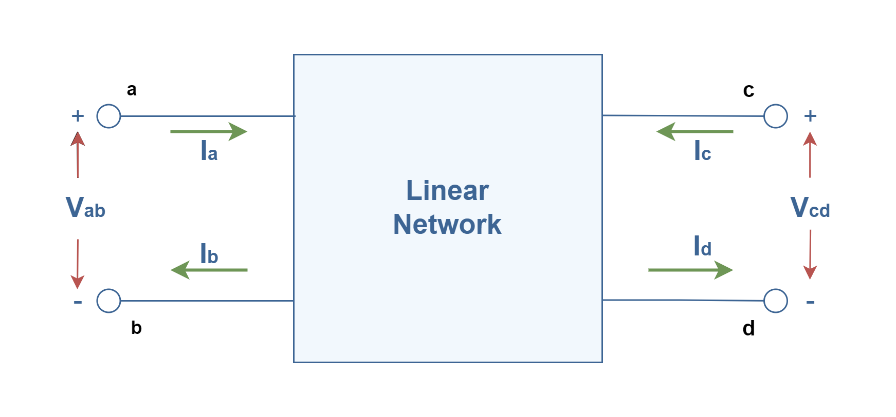
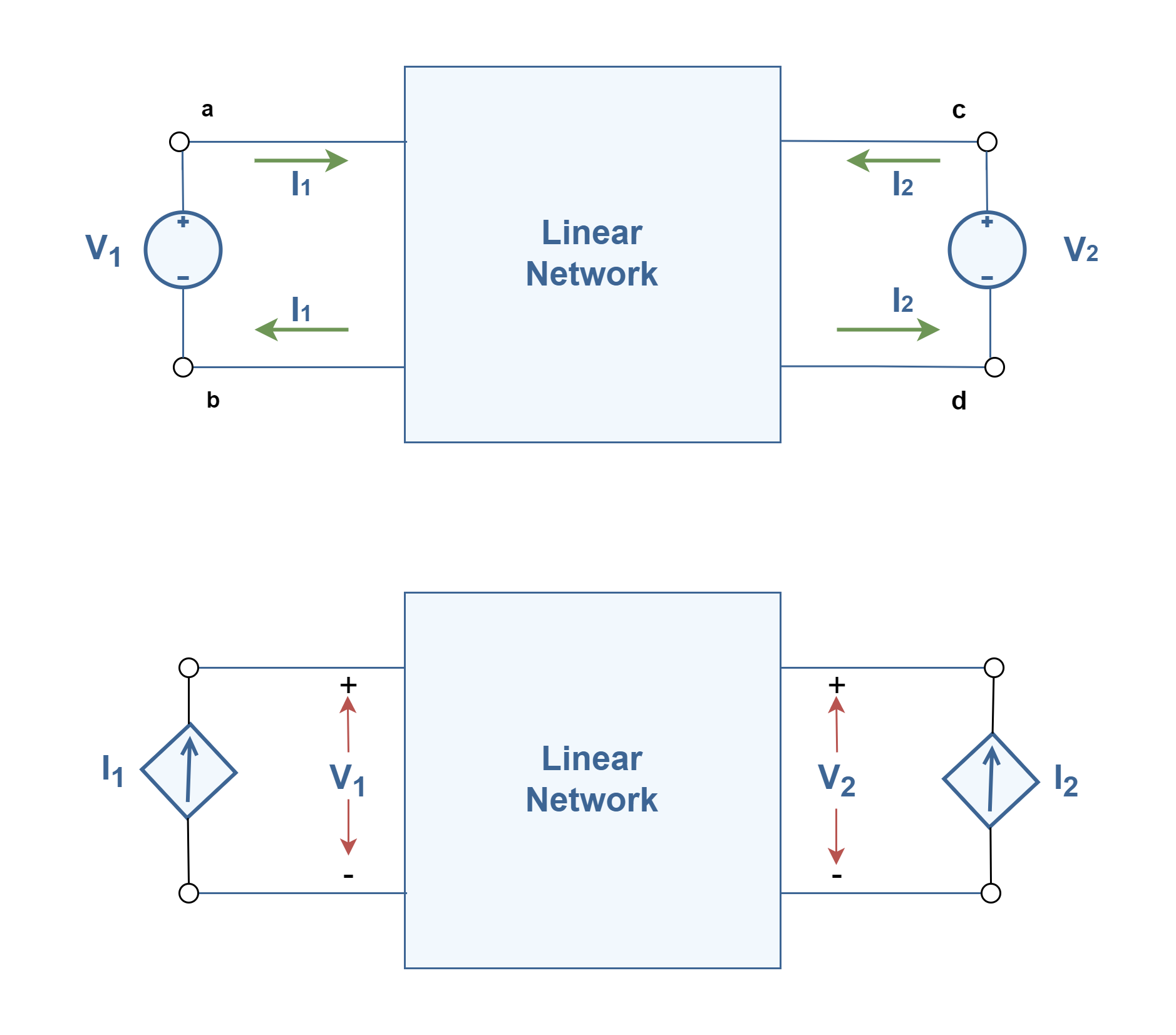
Each circuit normally accepts an input signal at a set of terminals and produces an output signal at a set of other terminals. Basically, a two-port network has two terminal pairs acting as access points, as shown in Figure 3, the current enters one terminal of each pair, ‘a’ and ‘c’, and leaves the other terminal in each pair, ‘b’ and ‘d’. Here we see the input port, represented by V_ab and I_a (or I_b), and the output port, represented by V_cd and I_c (or I_d). It should be noted that the representation of currents and voltage in two ports are based on sign conventions in electrical circuits. The same restrictions about external connections and internal sources mentioned above for the single port systems are also applied.

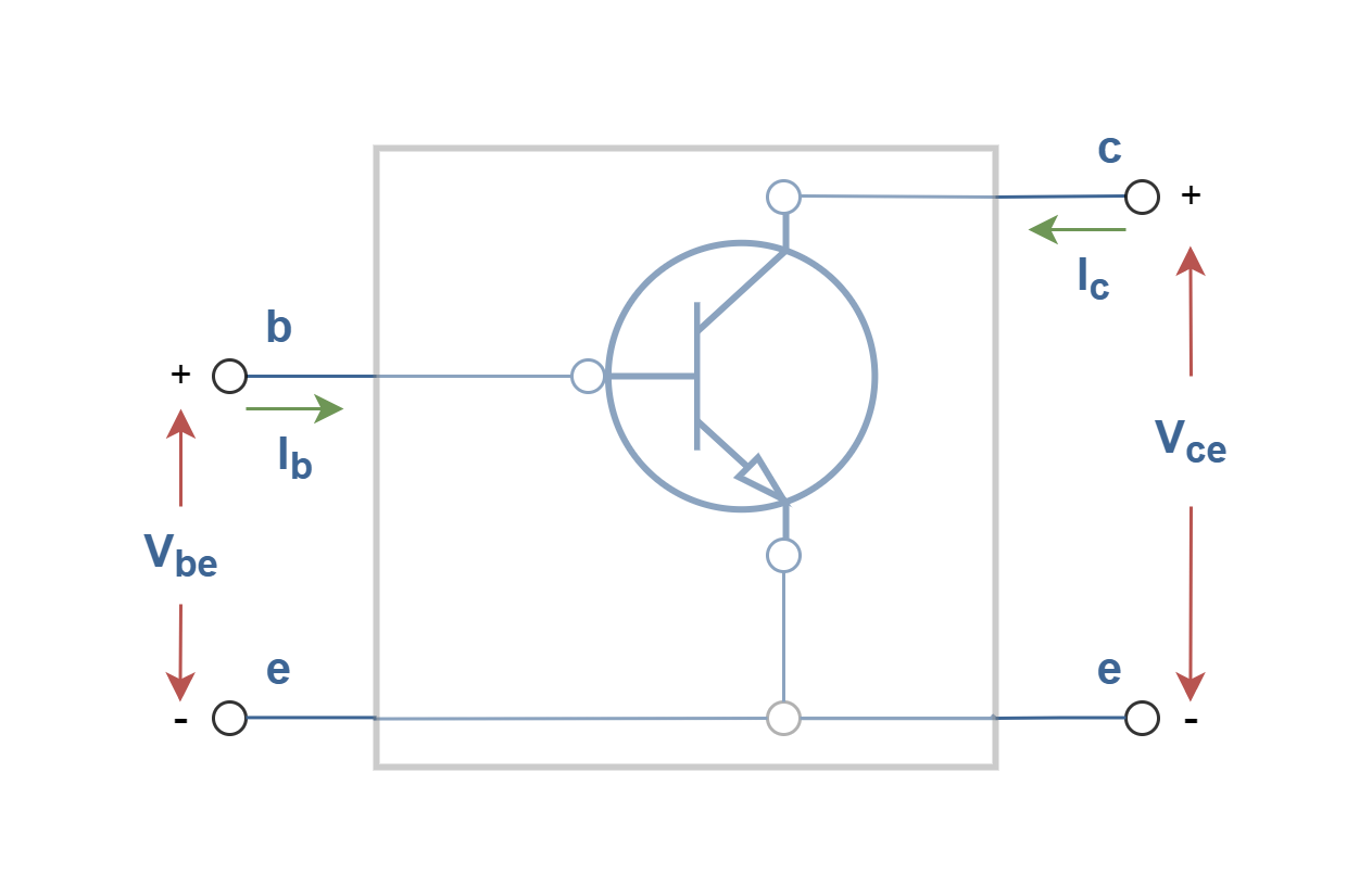
For example, a bipolar transistor as a three-terminal device in a common-emitter configuration can be used as a linear amplifier, has an input port between its base and emitter (V_be and I_b) and an output port between the collector and emitter (V_ce and I_c); as shown in Figure 4. Essentially, the transistor action can be described such that the voltage across two terminals (base and emitter) controls the current in the third terminal (collector). We can also apply the two-port system model (Figure 3) in such circuit. This is also applicable to other electronic active or passive devices like op-amps and transformers.

Mathematical demonstration of two-port networks is important because such circuits are used in huge applications like communications, control, and power systems. Additionally, knowing the parameters of a two-port network enables us to consider it as a black box when embedded within a larger network i.e., this reduces the analysis complexity.

Mathematical Modeling Of Two-port Networks Based On Z-parameters

There are many options to establish a model. Here, just the z-parameter (impedance) technique is introduced. In order to produce a mathematical model of circuits represented by a two-port linear network, we must find relationships between voltages and currents. Let us visualize placing two voltage sources at the input and the output, as shown in Figure 5. Thus, we have selected two of the variables, V₁ and V₂. We call these variables the independent variables. The remaining variables, I₁ and I₂, are dependent upon the selected applied voltages. We call I₁ and I₂ the dependent variables. (Also it is possible to imagine there are 2 current sources placed in the input and output ports i.e., the type of variables will be interchanged).

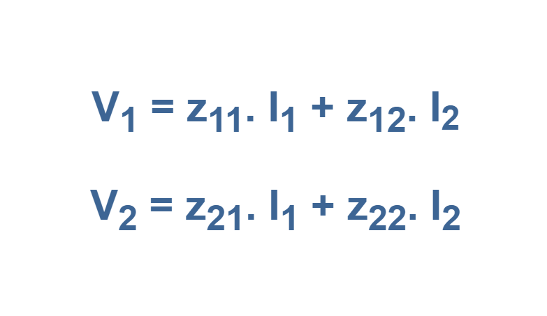
To analyze the system, we use the principle of superposition which states: The response of a linear circuit excited by multiple independent input signals is the sum of the responses of the circuit to each of the input signals alone. Using superposition method, we can write each dependent variable as a function of independent variables as follows in Equation 2:

In Equation 2, the coefficients of z_ij are called as parameters of the two-port network. These parameters can be calculated by setting input port or output port in open-circuited condition i.e., by disconnecting sources simply. Equation 3 shows the set of equations which used for computation. Since the parameters are found by setting port currents, I₁ or I₂, equal to zero, they are called open-circuit parameters. Also, since the definitions of the parameters as shown in Equation 3 are the ratio of voltages to currents, they are referred as impedance parameters, or z-parameters.

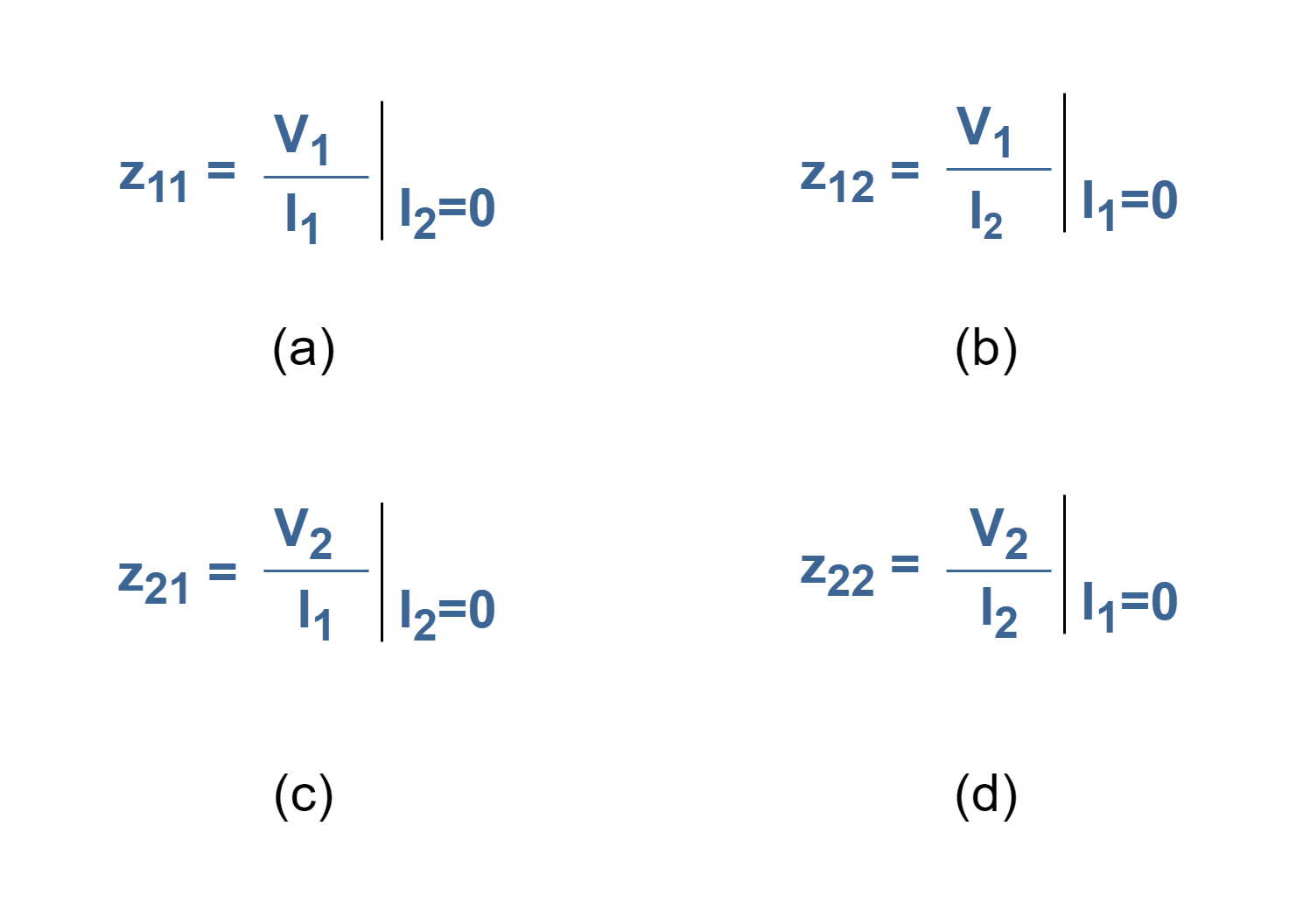
By these definitions we can call z-parameters new characteristics:

• z₁₁ as the input impedance of the linear network;
• z₁₂ as the transfer impedance from port 1 to port 2;
• z₂₁ as the transfer impedance from port 2 to port 1;
• z₂₂  as the output impedance of the linear network.

Many real two-port networks appear in the configuration like Figure 6 in which one port delivers energy by voltage or current sources i.e., the excitation is generally applied at this input port, and the other port consumes energy i.e., it normally extracts the desired signal by a load.  The symbol of Z_S indicates the internal impedance of the voltage source and Z_L indicates the impedance of the external electrical load.

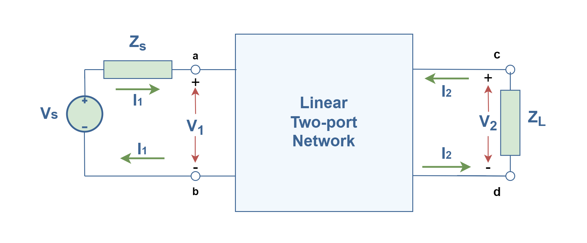
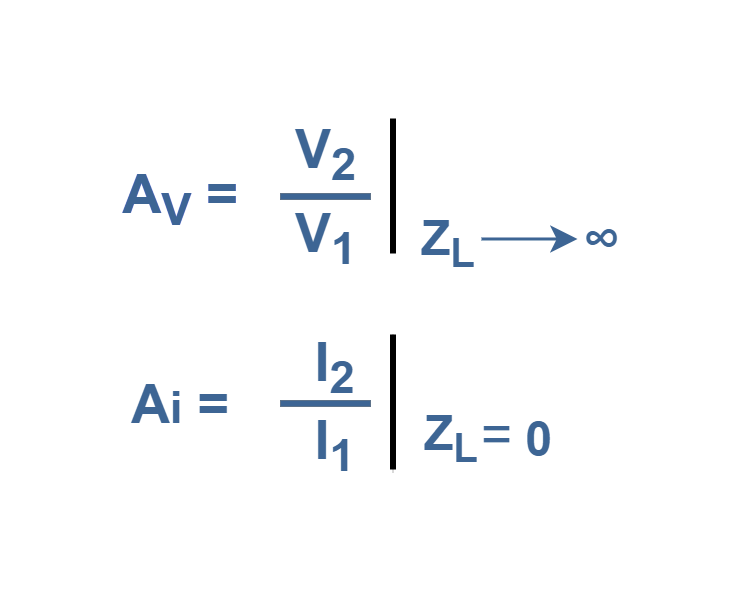
In such configurations, which are very common in amplifier systems, it is possible to define the gain of voltage (or current) between input and output ports. we can specify two important definitions for gains of the two-port network as shown in Equation 4. In this set of equations, A_v stands for network (open-circuit) voltage gain and A_i stands for network (short-circuit) current gain.

The amplifiers take power from an external source of energy (normally a DC power supply) and use it to boost the input signal. Finally, the amplifier delivers an output signal whose waveform corresponds to the input signal but its power level is higher. The output waveform of an amplifier must be an exact duplication of the input waveform. It preserves the details of the signal waveform and any deviation of the output waveform from the shape of the input waveform is considered as distortion.

Frequency Response Of A Two-port Network

The frequency response characteristics of a system can be found directly from its transfer function. Normally in each amplifier the response of gain magnitudes, |A(jω)|, verses frequency ranges can be plotted in logarithmic scale similar to the graph in Figure 7. The values of amplitude are in terms of Decibels (dB) and frequency values are measured in Hertz (Hz).

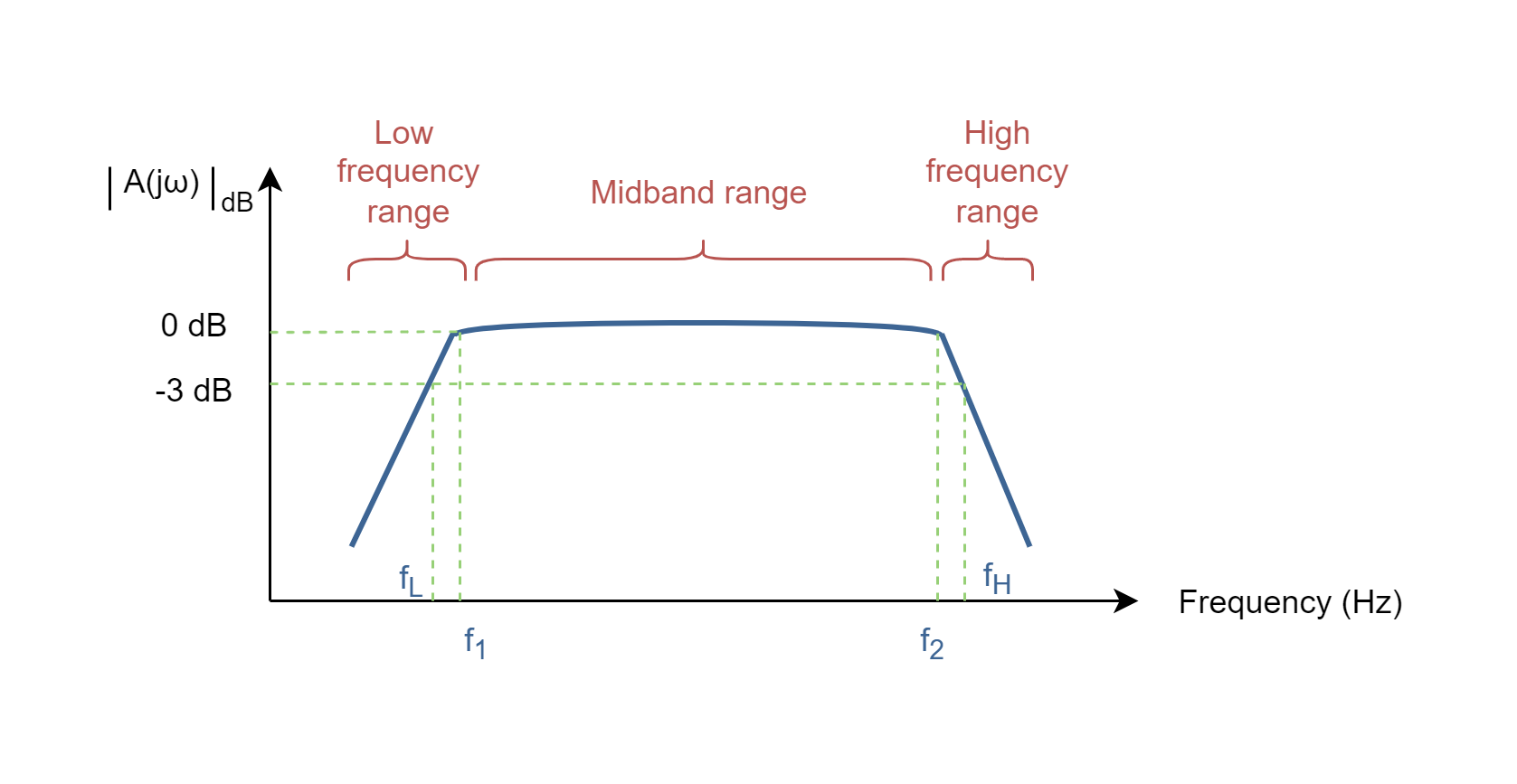
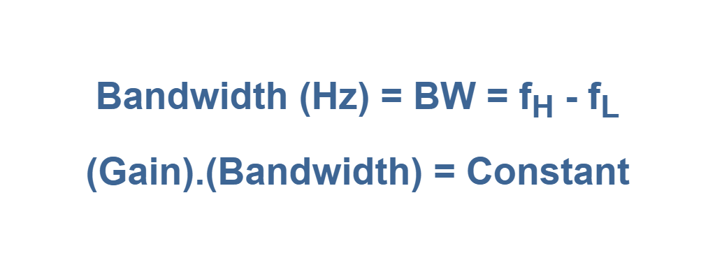
For a practical amplifier the gain drops off at high frequencies due to the active device and circuit capacitances. Gain may also drop off at low frequencies for capacitive coupled amplifier stages. Three frequency ranges are indicated in the Plot: low, midband and high frequency ranges. If the linearity would be critical in the performance of the system, the ideal operating region could be between frequencies of f₁ and f₂, in the midband range, because of perfect flat response. But, for most of amplifier systems the operation between frequencies of f_L and f_H would be acceptable, where the gain of the system is almost constant. The value of gain at f_L and f_H is 3 dB less than the maximum midband gain (0 dB in the graph). f_L and f_H are called the lower and upper corner (cut-off) frequencies, respectively. The Bandwidth of the amplifier stage is the difference between these 2 high and low frequencies as shown in Equation 5.

There is a Figure of Merit applied to amplifiers called the Gain-Bandwidth Product (GBP) that is commonly used to initiate the design process of an amplifier. It provides important information about the relationship between the gain of the amplifier and the expected operating frequency range.

Summary

• Many networks can be considered as having two pairs of terminals: a pair of input terminals at which the excitation is usually applied, and a pair of output terminals at which the desired signals are extracted. Because the system behaves linearly, the variables are related by a set of linear equations. These equations relate the port currents and voltages and define a set of two-port parameters.
• The functions of each two-port linear network can be described with mathematical models based on measures of each terminal. One of the simple and well-known models is the z-parameters model which is based on impedance parameters between terminals of the network.
• Voltage and current gains are also defined for linear two-port networks.

Please follow and like us: