Magnetostatic Fields In Material Bodies

The Magnetic Dipole Moment

Magnetostatic fields in material bodies represent a fascinating intersection of electromagnetic theory and material science. Unlike magnetic fields in a vacuum, which depend just on the distribution of currents, magnetic fields within materials are significantly influenced by the material’s intrinsic properties. At first, we need to introduce a concept that helps us to consider how different materials respond to and modify magnetic fields.

According to Ampere’s model, a small current loop that can produce a magnetic field is called a magnetic dipole. The magnetic dipole moment (M_d) is a measure of the magnetic strength and orientation of a magnetic dipole.

The dipole moment M_d is defined as equal to the product of the area of the plane current loop and the magnitude of the circulating current. The direction of the vector M_d is that of the normal vector n to the plane of the current loop and thus is given by the second right-hand rule.

Figure 1 shows the magnetic dipole and its moment vector in a 3D Cartesian coordinate.

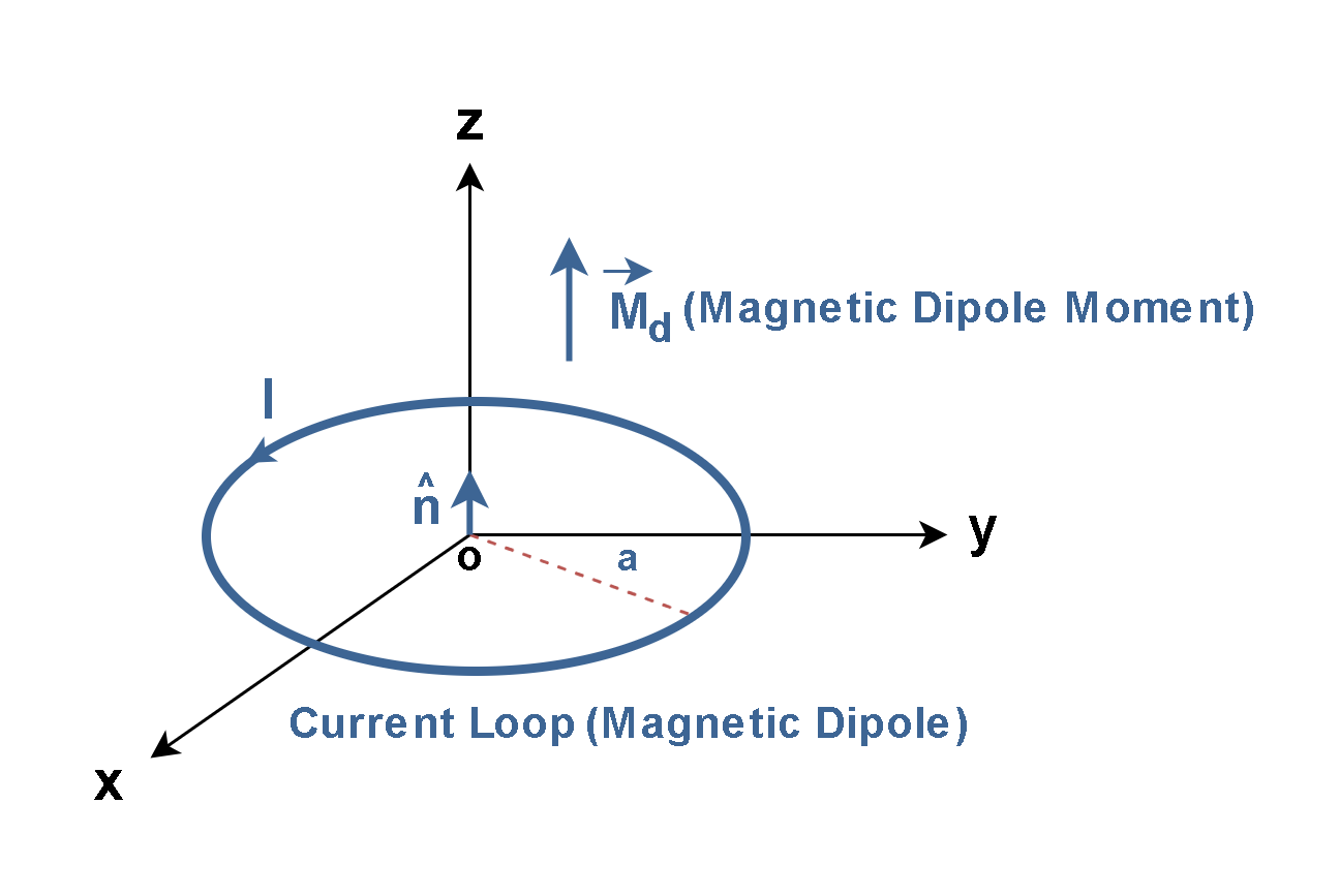
For a circular loop of radius ‘a’, the magnitude of the dipole moment is defined by Equation 1:

where n̂ is the unit vector perpendicular to the loop. The SI unit for magnetic dipole moment is ampere-square meter (A·m²) or joules per tesla (J/T).

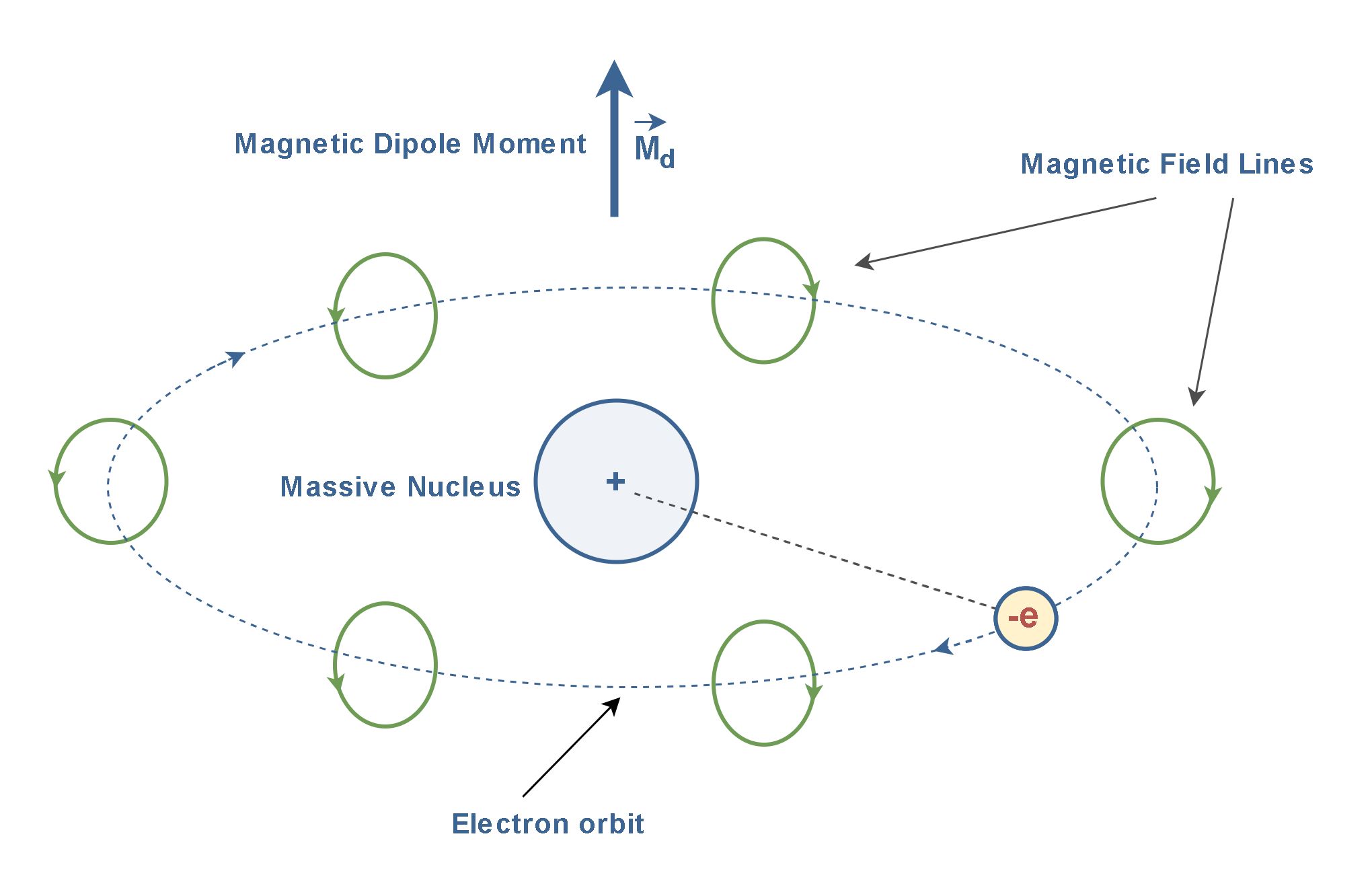
According to the atomic theory, all matter is composed of a number of basic elementary particles, of which the electron, proton, and neutron are perhaps the best known. These particles combine to form atoms, which we may think of as a nucleus as a collection of neutrons and protons into a central heavy core around which a number of electrons rotate along closed orbital paths. The electrons rotating in orbital paths are equivalent to circulating current loops on an atomic scale.

In particular, an individual atom should act as a small magnet, with a north pole and a south pole, because of the motion of the electrons about the nucleus, as Figure 2 illustrates.

The magnetic properties of many materials can be explained by the fact that an electron not only circles in an orbit, but also spins on its axis, with spin magnetic moment as Figure 3 illustrates (recall that the charge is negative).

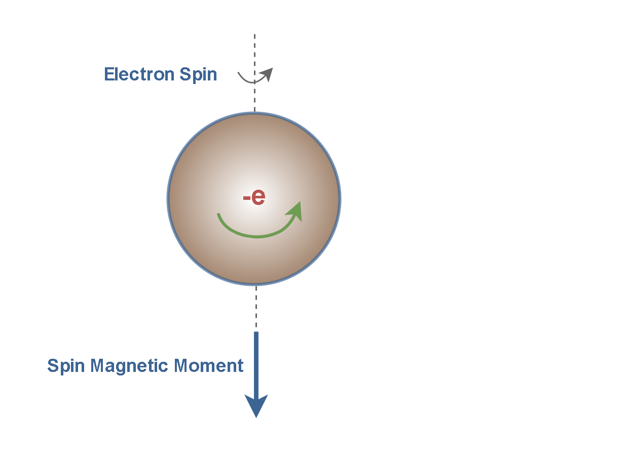
The spinning electron represents a charge in motion that also produces a magnetic field. The field due to the spinning is generally stronger than the field due to the orbital motion.

Essentially, there are two main properties of atoms that give rise to magnetic dipole moments:

1. Electron orbital motion around the nucleus (orbital magnetic moment)
2. Electron intrinsic spin (spin magnetic moment)

However, the magnetic field produced by one electron in an atom is often canceled by an oppositely revolving electron in the same atom. Then, the net result is that, for most materials, the magnetic effect produced by the electrons orbiting the nucleus is either zero or very small. That is why most substances are not magnetic.

Table 1 presents approximate magnetic dipole moments for a few notable physical systems, measured in joules per tesla (J/T).

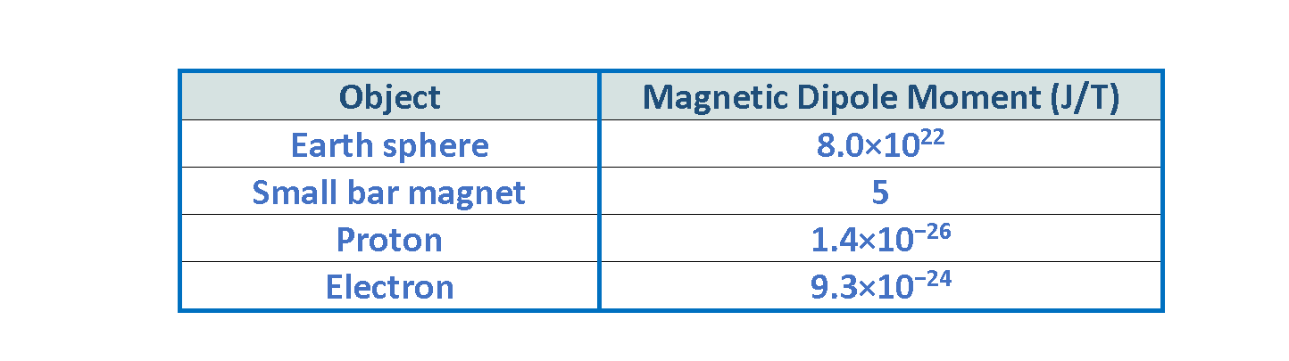
This table emphasizes the vast range of magnetic dipole moments found in nature—from sub-atomic particles (with very small moments), to large-size macroscopic objects (with large moments).

Magnetization Mechanism In Materials

We can consider a material body of volume V that is bounded by a surface S, as in Figure 4.

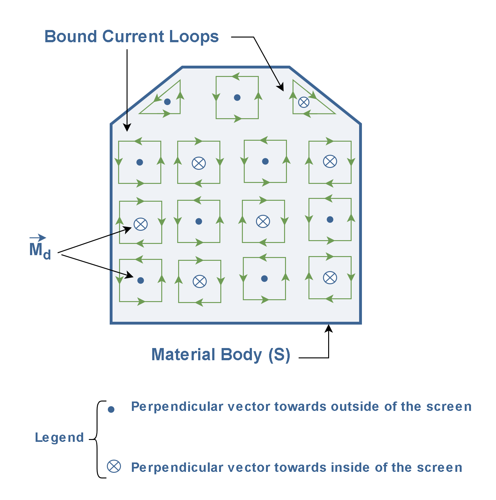
We may think of this material body as consisting of a large number of small circulating current loops that we may treat as microscopic magnetic dipoles. They have magnetic dipole moments M_d. These molecular current loops were proposed by André-Marie Ampère, a 19^th-century French physicist, are known as bound currents. Bound currents are not actual free-flowing currents like those in a wire, but rather a conceptual tool to describe magnetization effects. The field due to magnetization of the medium is just the field produced by these bound currents.

In most materials at normal temperatures and in the absence of an external magnetic field, thermal agitation causes the atomic magnetic dipoles to be randomly oriented, resulting in zero net magnetization.

When a material is placed in an external magnetic field B_ext ​, the magnetic moments tend to align with it, creating a net magnetization vector M, which represents the magnetic dipole moment per unit volume, as explained by Equation 2.

where ∑ M_d is the sum of all microscopic magnetic moments in volume V. So, the magnitude of magnetization (M) can be thought of as the density of microscopic magnetic dipole moments throughout the material. The vector M is measured in amperes per meter (A/m).

Figure 5 shows an arbitrary material body after being placed in an external magnetic field B_ext.  In this thin slab of uniformly magnetized material, the dipoles are also represented by tiny current loops. The blue arrows represent the orientation of magnetic dipole moments.

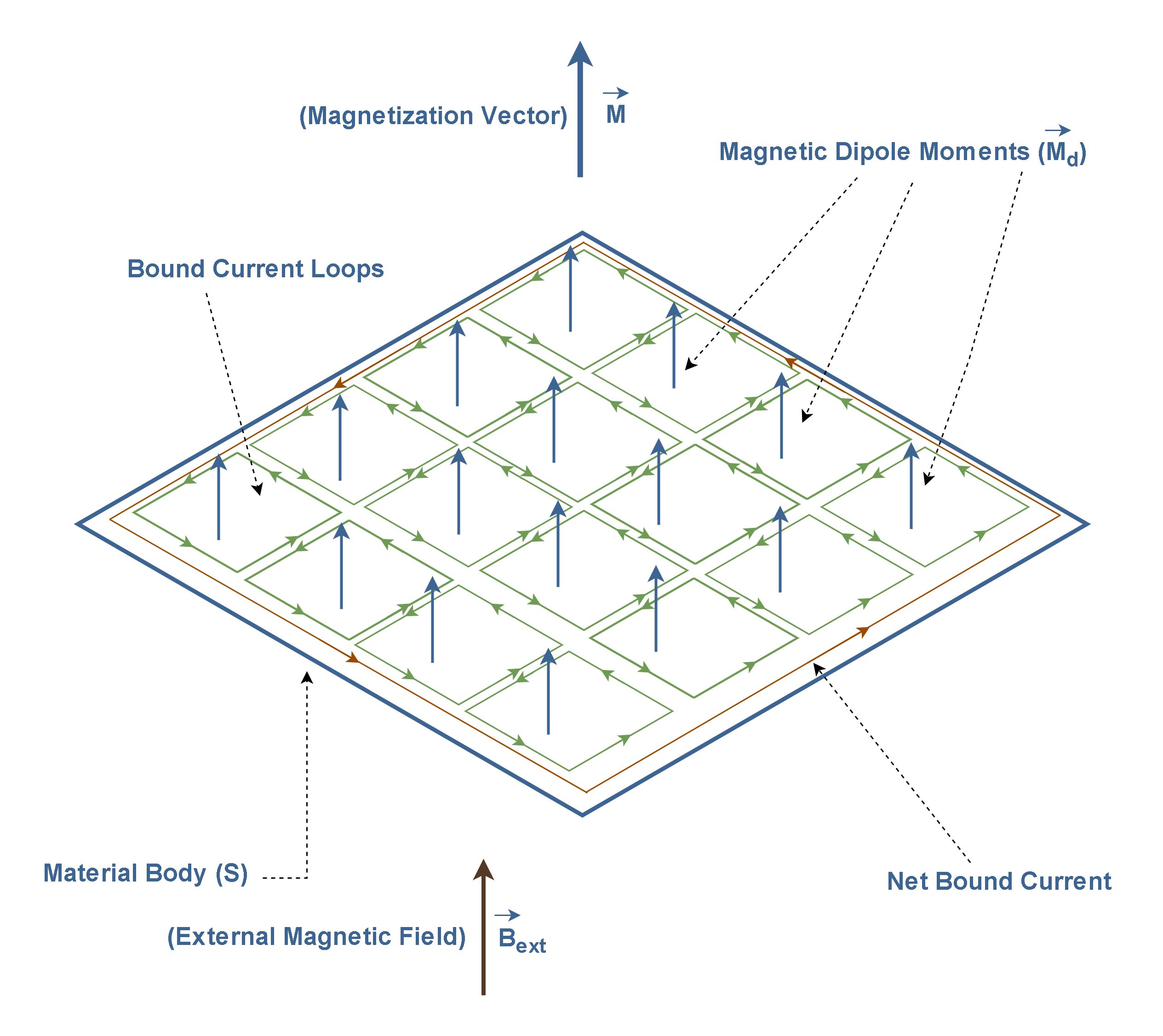
Note that all the “internal” currents cancel each other out: every time one goes to the right, another one, next to it, goes to the left. However, at the edges, there are no adjacent loops to do the canceling. The whole thing, then, is equivalent to a single path of net-bound current flowing around the boundary.

Essentially, when materials are present, we need to separate the contributions to the magnetic field B_ext into two categories:

• Contributions from free-flowing currents (which we can control)
• Contributions from the material’s response (intrinsic magnetization mechanism)

Free currents are ordinary conduction currents flowing on macroscopic paths – currents that can be started and stopped with a switch and measured with an ammeter.

Therefore, in any material, the total current can be written as Equation 3:

where the free current I_free involves actual transport of charge and the bound current I_bound results from many aligned atomic dipoles.

So, we can express the total magnetic field in the material as the field attributable to bound currents, plus the field due to the free current. Equation 4 simply explains this fact:

where B_free is the field due to the true current and B_bound is the field due to the surface-bound current around the sample.

The Magnetic Field Intensity H

Magnetic field intensity (H) is an alternative description of the magnetic field B in which the effect of the material is factored out.

H represents the magnetic field that would exist if all materials were removed but free currents remained, while B represents the actual magnetic field including material effects.

H has a close relationship with free current. The relationship between B and H is explained by Equation 5:

where:

• B is the total magnetic flux density (measured in tesla, T)
• H is the magnetic field strength (measured in amperes per meter, A/m)
• M is the magnetization of the material (also in A/m)
• μ₀ is the permeability of free space (4π × 10⁻⁷ H/m)

The quantity of vector H is defined by Equation 6:

Ampere’s Law In Magnetized Materials

The magnetic field intensity (H) permits us to express Ampere’s circuital law in terms of the free current alone, and the free current is what we control directly.

Figure 6 shows a bar of a conductor carrying a steady current ‘I₀’ while the magnetic field strength vector H encircles the current tangent to a closed loop. dl is a vector whose magnitude equals to an infinitesimal length of the loop and its direction is the same as H.

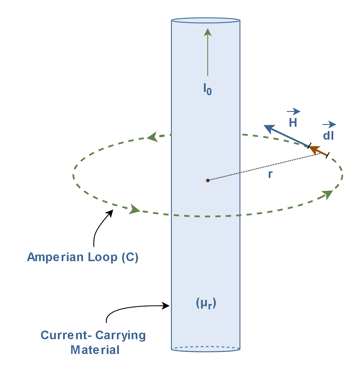
Then, Ampère’s circuital law can be written in integral form as Equation 7:

where:

• ∮ represents the line integral around a closed loop C.
• H is the magnetic field strength (measured in A/m)
• dl is an infinitesimal vector element of the loop in units of meters.
• I₀ is the total free current passing through the Amperian loop in units of amperes.

So, Equation 7 clearly shows that the magnetic field intensity (H) and steady I₀ are directly proportional. In particular, when symmetry permits, we can calculate the magnetic field intensity (H) immediately from the free current by Equation 7.

Types Of Magnetic Materials

Magnetic materials can be classified according to how they react to the application of an external magnetic field:

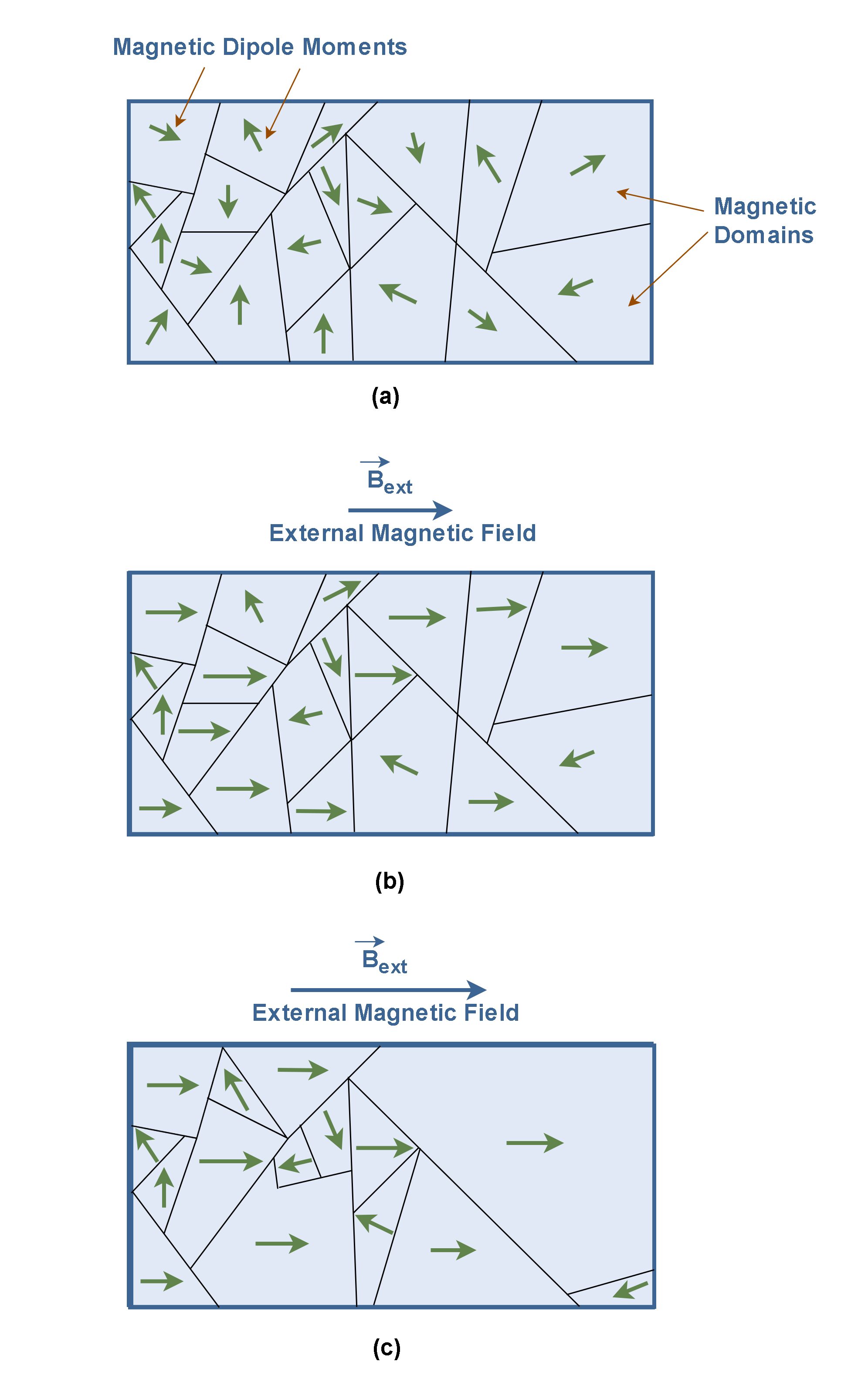
• In ferromagnetic materials, the atoms have permanent magnetic moments that align readily with an externally applied magnetic field. Examples of ferromagnetic materials are iron, cobalt, and nickel. Common magnets are also made of a ferromagnetic material. Such substances can retain some of their magnetization even after the applied magnetic field is removed. Experiments reveal that a ferromagnetic material consists of tiny regions known as magnetic domains. Their volumes typically range from 10⁻¹² to 10⁻⁸ m³, and they contain about 10¹⁷ to 10²¹ atoms. Within a domain, by coupling between neighboring atoms, the spins of electrons are aligned, and then the magnetic dipoles are also rigidly aligned in the same direction. This coupling, which is due to quantum mechanical effects, is so strong that even thermal agitation at room temperature cannot break it. The result is that each domain has an exact dipole moment. In an unmagnetized substance, the domains are randomly oriented, and there is no net magnetic dipole moment associated with the material, as shown in Figure 7a. If a sample of the ferromagnetic material is placed in an external magnetic field B_ext, some of the magnetic dipoles tend to line up parallel with the external field, as shown in Figure 7b. Since each dipole produces its own magnetic field, this alignment contributes an extra magnetic field, which enhances the applied field. It means the magnetic field B_total inside the material becomes larger than the external field (B_total > B_ext).  As the external field B_ext is made even stronger (Figure 7c), the domains that are not aligned with the external field become very small, and the aligned domains become larger. Consequently, the field due to the alignment of the domains is also quite larger. It causes the magnetic field B_total produced inside the material become completely stronger than the external field. Ferromagnets, like iron, retain their magnetization even after the external field has been removed.

• Paramagnetic materials also have permanent magnetic dipole moments that tend to align with an externally applied magnetic field, but the response is extremely weak compared with that of ferromagnetic materials. In paramagnetic materials, the spin and orbital magnetic dipole moments of the electrons in each atom do not cancel but add vectorially to give the atom a net (and permanent) magnetic dipole moment. In the absence of an external magnetic field, these atomic dipole moments are randomly oriented, and the net magnetic dipole moment of the material is zero. If a sample of the paramagnetic material is placed in an external magnetic field B_ext, only a small number (roughly one-third) of the magnetic dipoles are aligned with the applied field. It means the magnetic field in the material is increased by only a small amount. After magnetization by an external magnetic field, once the field is removed, thermal agitation produces motion of the domains, and the material quickly returns to an unmagnetized state. Examples of paramagnetic substances are aluminum, calcium, and platinum.
• The diamagnetic materials do not have any permanent magnetic dipole moments in the absence of an external applied magnetic field. In diamagnetic materials, an externally applied magnetic field induces a very weak magnetization (magnetic dipole moment) that is opposite the applied field. This results in a net magnetic field in the interior of the material body, which is less than that of the external field itself (B_total < B_ext). Some of the materials in this class are copper, bismuth, zinc, silver, lead and mercury.

Briefly, in paramagnetic and ferromagnetic materials, the induced magnetic dipoles are masked by much stronger permanent magnetic dipole effects of the atoms. However, in diamagnetic materials, whose atoms have no permanent magnetic dipoles moments, the effect of the induced dipoles is more observable.

Magnetic Susceptibility And Permeability

In paramagnetic and diamagnetic materials, the magnetization is sustained by the external field; when B_ext is removed, M disappears. In fact, for most substances the magnetization is linearly proportional to the field, provided the field is not too strong. This proportionality is stated by Equation 8:

The constant of proportionality Χ_m is called magnetic susceptibility. It is a dimensionless quantity that varies from one substance to another, positive for paramagnetic and negative for diamagnetic materials. Typical values are explained for some materials in Table 2:

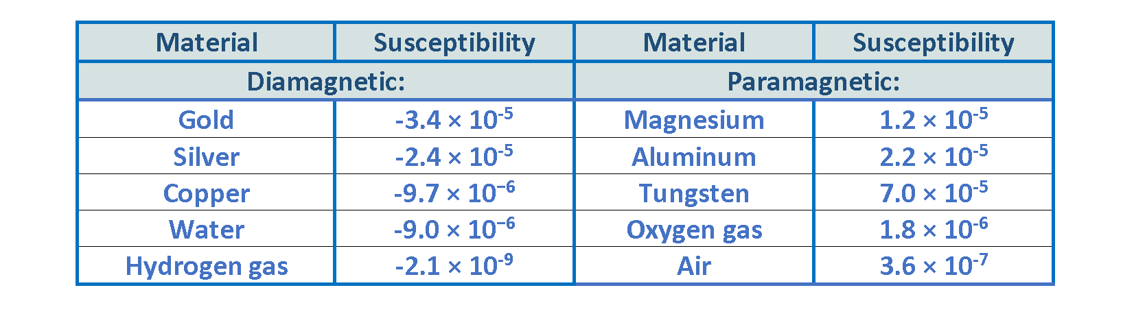
Materials that obey Equation 8 are called linear media. Note that ferromagnetic materials are generally non-linear, which is why they are not included in Table 2.

For linear media, B is also proportional to H by Equation 9:

where μ is called the permeability of the material. Equation 10 also explains the relationship between permeability and susceptibility of a material:

In a vacuum where there is no matter to magnetize, the susceptibility vanishes, and the permeability is μ₀, which is called permeability of free space: μ₀ = 4π × 10⁻⁷ H/m (Henries per meter)

Permeability describes the effect of a material in determining the magnitude of the magnetic field (B). All else being equal, B increases in proportion to permeability.

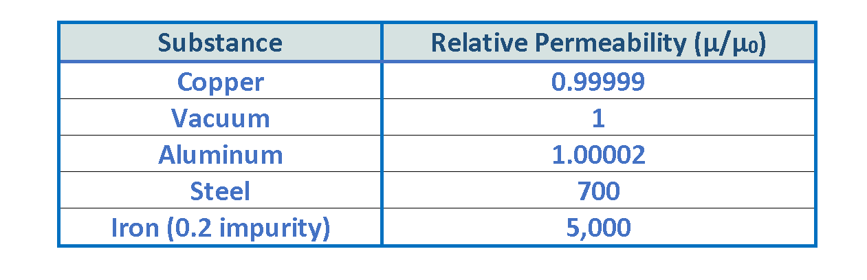
It is common practice to describe the permeability of materials in terms of their relative permeability (μ_r,) which gives the permeability relative to the minimum possible value; i.e., that of free space. Equation 11 introduces the quantity of μ_r:

Table 3 provides values of the magnetic relative permeabilities of some substances:

Application Of Ferromagnetic Materials In Electromagnets

An electromagnet is a type of magnet in which the magnetic field is produced by an electric current. A simple way in practice to make an electromagnet is to wrap a coil of wire around a ferromagnetic object (like the metallic part of a screw driver) which becomes magnetized when current flows (Figure 8). A current through the wire creates a magnetic field that is concentrated along the center of the coil.

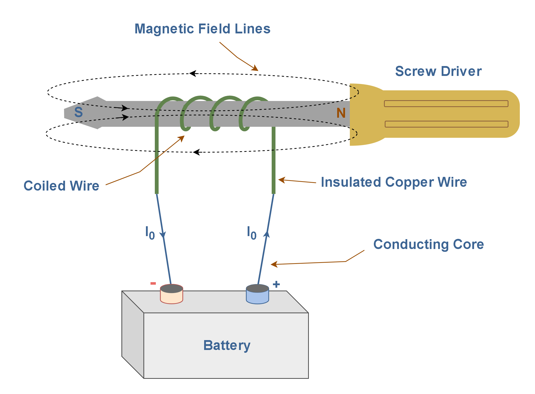
Firstly, the object contains an enormous number of domains, and their magnetic fields cancel, so it is not magnetized. We can run a current ‘I₀’ through the coil; this provides the external magnetic field, which is pointing from left to right inside the core in Figure 8.

Because the bound currents in the material inserted inside the coil (iron) tend to reinforce the free currents, the result is to strengthen the field. After magnetization, the screwdriver is able to absorb some other small particles of ferromagnetic materials.

Conclusion: Key Differences In Applications

If we compare ‘iron’ and ‘copper’ according to their intrinsic electrical and magnetic properties, we can find these facts: ‘iron’ and ‘copper ’ have similar electrical properties and their conductivity (σ) is almost in the same range. But, iron has a very high relative permeability (μ_r), typically in the range of 5000, depending on purity and processing. This makes iron excellent for magnetic cores and transformers. However, copper has a relative permeability very close to 1, meaning it’s practically non-magnetic. This is why copper isn’t used in applications requiring magnetic properties.

The dramatic difference in permeability means these metals serve completely different roles in electromagnetic applications:

• Iron is used where magnetic field amplification is needed: transformer cores, electric motors, inductors, and electromagnets.
• Copper is ideal where conductivity without magnetic interference is required: wiring, transmission lines, and electronic components.

Summary

• Magnetic dipole moment arises from a current loop; direction follows the right-hand rule.
• Atoms behave as magnetic dipoles due to: electron orbital motion and electron spin.
• The orbital motion of electrons around the nucleus is equivalent to a circulating current loop.
• Most materials have no net magnetization due to random dipole orientations.
• Net magnetic behavior arises when dipoles align under an external field.
• Materials are modeled as many small current loops, i.e., bound currents.
• Aligned dipoles produce surface-bound currents forming a net field.
• Bound currents produce their own magnetic fields that contribute to the total field.
• We cannot turn bound currents on or off independently, as we can do by free currents.
• Magnetic field intensity H can be computed directly from a distribution of current using the Ampere’s law.
• In the absence of any external applied magnetic field, the magnetic dipoles of individual atoms are randomly oriented and the body as a whole will have a zero net magnetic moment.
• When a ferromagnetic material is placed in a magnetic field, its magnetic dipoles also become aligned with the field. Then, the medium becomes magnetized.
• The alignment occurs in relatively small patches, called domains.
• Domains become locked together so that a permanent magnetization results, even when the external field is turned off.
• Paramagnetic materials have some permanent magnetic dipole moments, but they have weak alignment with the external field and small enhancement of external field.
• An external magnetic field always induces a magnetic dipole in an atom.
• Diamagnetic materials have no net magnetic dipole moment. They produce a weak opposing induced field after applying an external magnetic field.
• Electromagnets use a coil wound around ferromagnetic cores to amplify the magnetic field B.

Please follow and like us: