Effects Of Magnetic Fields In Vacuum

The Biot-Savart Law In Magnetostatics

The Biot-Savart law is one of the fundamental laws in magnetostatics that describes how electric currents produce magnetic fields. Named after French physicists Jean-Baptiste Biot and Félix Savart, who discovered it in 1820, this law provides a way to calculate the magnetic field at any point in space due to a current-carrying wire.

Figure 1 shows an arbitrary loop (C) of steady current (I). We can select dl as an element of length along the wire and r^ as the unit vector pointing from the wire element to the observation point P, where we calculate the magnetic field.

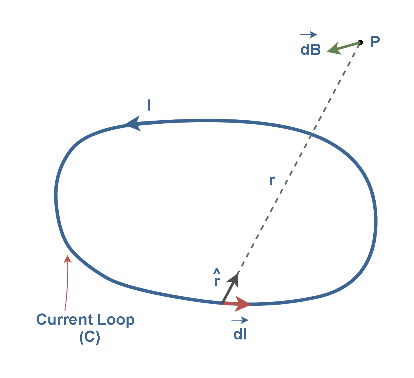
The magnetic field element dB of a steady current ‘I’ is generally given by the Biot-Savart law as shown in Equation 1:

where:

• dB is the differential contribution to the magnetic field in units of tesla
• μ₀ ​ is the magnetic permeability of free space (4π × 10⁻⁷ Henry per meter)
• I is the current in the wire in units of ampere
• dl is a differential element of the wire measured in meters
• r^ is the unit vector pointing from the source to the observation point
• r is the distance from the wire element to the observation point ,measured in meters

To find the total magnetic field B, we integrate Equation 1 over the entire current distribution. So, the integration is along the current path ‘C’, in the direction of the flow as explained in Equation 2:

The magnetic field B is also called the magnetic flux density. The Biot-Savart Law states that each small segment of wire (dl) carrying current (I) contributes a small component to the magnetic field (dB) at point P. The total magnetic field B can be achieved by integration of all the small contributions.

The units are such that B itself comes out in newtons per ampere-meter or teslas (T): 1 T = 1 N/(A·m).

The Biot-Savart law tells us that:

1. The magnetic field strength (B) at any point is proportional to the current (I)
2. The field strength decreases with the square of the distance from the current source (r²)
3. The magnetic field circulates the current path, and its direction follows the second right-hand rule (RHR-2) that we will explain later.

This law can be used to calculate the magnetic field for various current configurations:

• Straight wires
• Circular loops
• Coils or Solenoids
• Any arbitrary current distributions

Figure 2 shows a wire carrying a steady current ‘I’ which produces circular loops of magnetic field lines.  A sketch of the magnetic circles is shown in Figure 2a from side view, while in Figure 2b there is a sketch from top view (cross-section perpendicular to the wire).

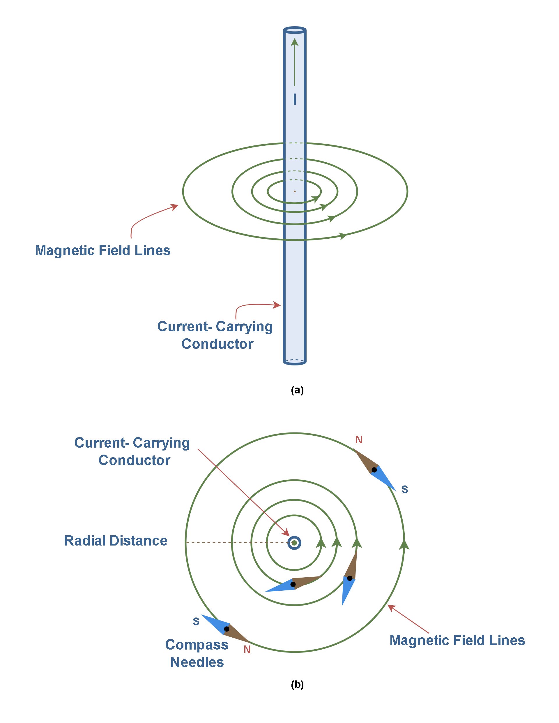
In Figure 2, the areas where the field lines are closer together indicate where the field is stronger. Although only some field lines are shown above, the field is technically present even infinitely far away from the wire. However, the strength of the field is negligibly small very far away. The reason is that the field strength decreases with distance from the wire.

Figure 2b shows how we can find the trajectory of magnetic field lines by using some compasses around the wire at different angles and at different radial distances to the wire. The direction of the magnetic field is taken to be the direction indicated as “north” (N) by the compass needle.

Essentially, when this field is explored with a compass needle, the magnetic field produces an aligning force on the needle such that the needle always orients itself normal to a radial line originating at the center of the wire. This orientation is parallel to the magnetic field. If one moves in the direction of the needle, it is found that the magnetic field forms closed circular loops around the wire.

In Figure 2b, the current in the wire is flowing out of the page. In drawing figures, if the current or magnetic field vector were coming out of the page, we represent this with a dot. If the current or magnetic field were going into the page, we represent this with a cross.

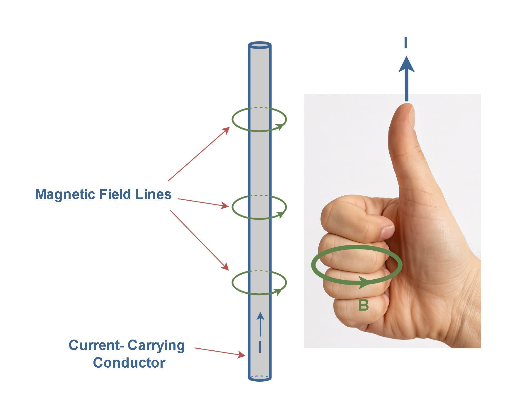
Recall that we already considered the first right-hand rule to find the direction of the magnetic force in the past articles. Now we use the second right-hand rule (RHR-2) to find the relation of the magnetic field direction to the current direction.

As Figure 3 shows, the rule, with the thumb pointing in the direction of the current, the fingers of the right hand encircle the wire in the direction of the magnetic field.

The Magnetic Field Of Special Arrangements Of Current-Carrying Elements

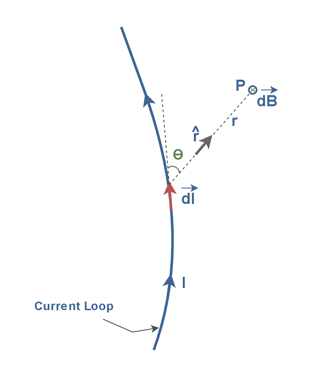
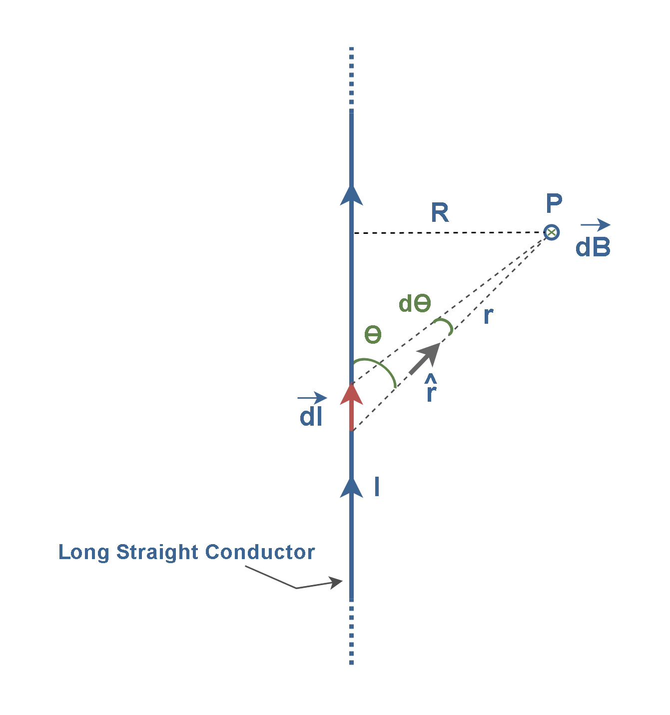
In Figure 4, in case we wish to know B at a point P, due to a current ‘I’ in a long curved conductor, we assume that the conductor is made up of elements or segments of infinitesimal length dl connected in series.

By the Biot-Savart law method, the total magnetic field B at the point P, is then the sum of the contributions from all differential elements dB, which are expressed by Equation 1. For clarity, we will focus on finding just the magnitude of the magnetic field vector B. Thus, Equation 3 calculates the total magnetic field B by integration of differential elements:

where:

• B is the magnetic field at P in units of T
• I is the current in the conductor, A
• dl is the length of the current element, m
• r is the distance from the element to P, m
• θ is the angle measured clockwise from the positive direction of current along dl to the direction of distance r extending from dl to P

The integration is carried out over the entire length of the conductor. The direction of vector B is inward at P and normal to the page.

Figure 5  shows the geometry of a long straight wire a current ‘I’ in which we want to find the magnitude of the magnetic field B at a radial distance R from a long conductor.

According to the right-hand rule, with the current I as indicated, B at the right of the wire is into the page. Based on Figure 5, since (dl.sin θ = r dθ) and (R = r sin θ), then Equation 3 in this case converts to Equation 4:

where the integration is between the angles θ = 0 and θ = π, that is, over the entire length of the long wire. Integrating gives us Equation 5:

Finally, Equation 6 is achieved:

The constant distance R appears in the denominator of the Equation 6 for the magnetic field strength. It means that B and R are inversely proportional to each other, and the magnetic field strength goes to 0 as R goes to infinity. Figure 6 shows the results of Equation 6 as a hyperbolic curve in terms of distance from a 1 amp current-carrying wire.

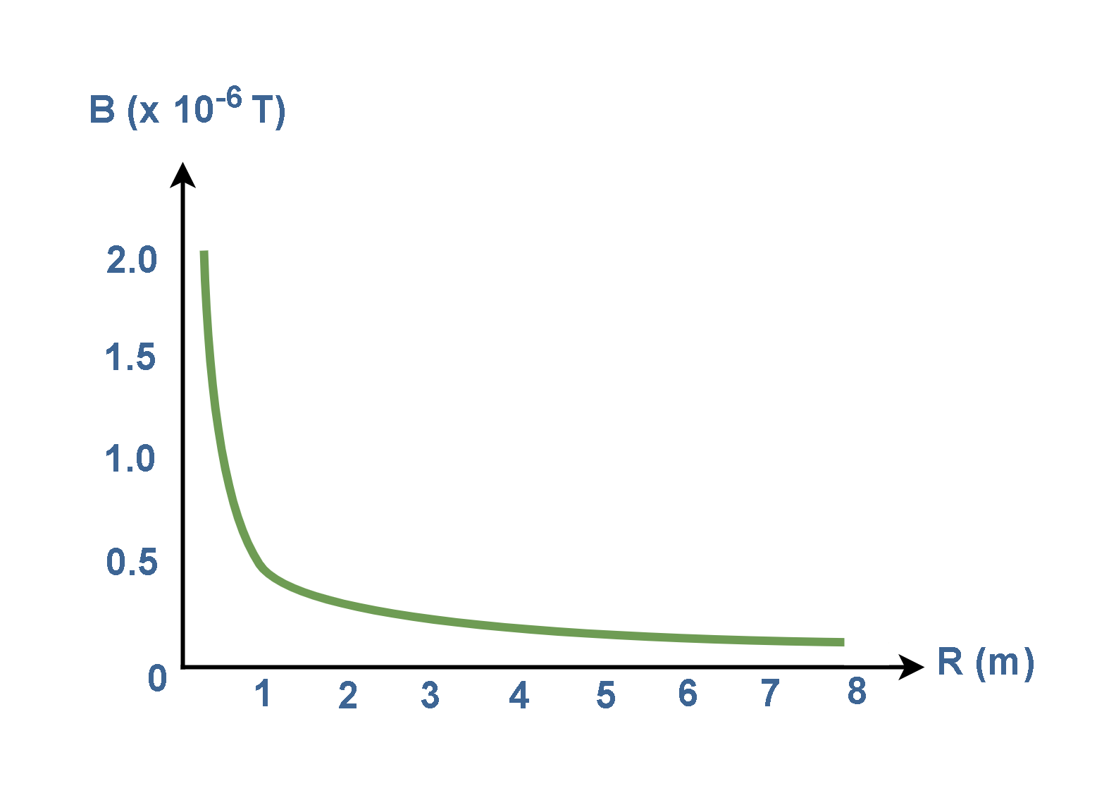
The graph shows that the field strength decreases rapidly in the space close to the wire (R < 1m) and gradually decreases as you move further away (R > 1m).

Relationship Between Laws In Magnetostatics And Electrostatics

As the starting point for magnetostatics, the Biot-Savart law plays a role analogous to Coulomb’s law in electrostatics. Indeed, the term (1/r²) is common to both laws.

A comparison between Biot-Savart law and Ampere’s laws (which we have already considered in the previous article) might also be valuable.

The Biot-Savart law and Ampère’s force law in magnetostatics are related. The Biot-Savart law calculates the ‘magnetic field’ due to a current element, while Ampère’s force law describes the ‘magnetic force’ between current-carrying conductors.

Ampère’s circuital law gives the magnetic field in terms of a line integral around a closed path, while the Biot-Savart law directly calculates the field at any given point.

While Ampère’s circuital law is often more convenient for highly symmetric situations to find the magnetic field, the Biot-Savart law is more general and can be applied to any current distribution, symmetric or asymmetric.

It is also worth mentioning that we have already achieved the same result of Equation 6 (based on Biot-Savart law) in this article with Equation 3 by using Ampère’s circuital law in the previous article.

Effect Of A Static Magnetic Field On A Current-Carrying Wire

In previous articles, we considered that moving charges experience a force in a magnetic field. If these moving charges are in a wire, the wire should also experience a force.

Figure 7 shows such a configuration where a current-carrying wire is placed in a static magnetic field B created by a permanent magnet. It must therefore experience a force F due to the field.

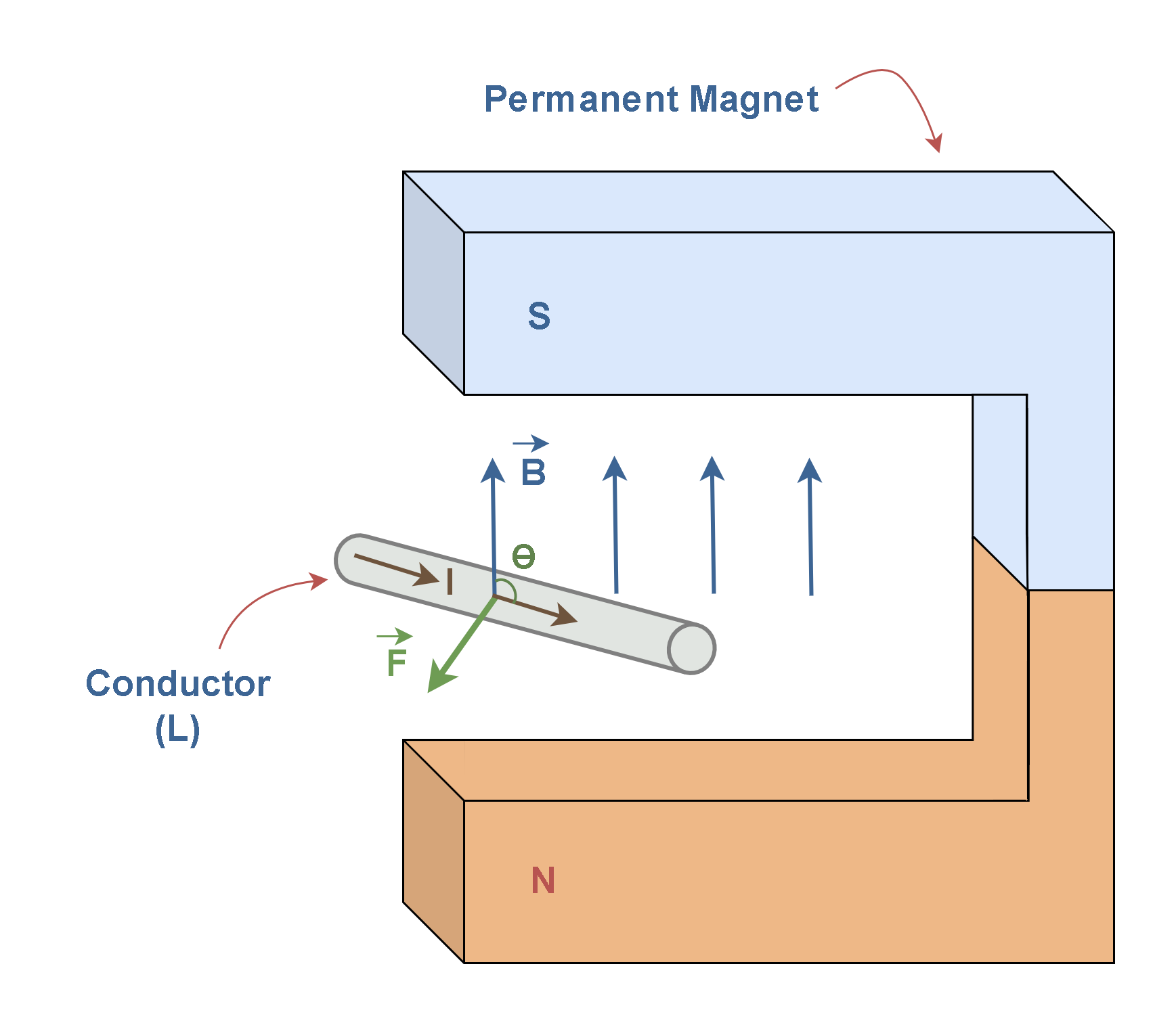
Consider the uniform magnetic field B between the poles N and S of the permanent magnet in Figure 7. The vectors of B and F are mutually perpendicular.

Generally, to investigate the magnetic force F, let’s consider the infinitesimal section of wire as shown in Figure 8. dl is a vector that represents the length and the direction of the section. The angle θ is measured clockwise from the positive direction of current along dl to the direction of the magnetic field vector B.

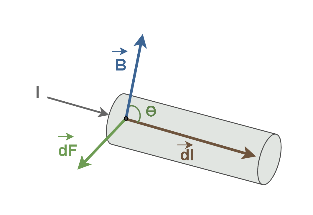
So, the magnetic force element on the charge carriers in the section of wire is dF, which is calculated by Equation 7:

This is the infinitesimal magnetic force on the section of wire. The direction of this force is given by the first right-hand rule (RHR-1), where you point your fingers in the direction of the current and curl them toward the magnetic field. Your thumb then points in the direction of the force. Then the force dF on the current element is normal to the plane containing vectors dl and B.

To determine the magnetic force on the whole wire, we must integrate Equation 7 over the entire length of the wire in a magnetic field (L). Because the wire section is straight and B is uniform, the differentials become absolute quantities, giving us Equation 8:

where:

• B is the uniform magnetic field in units of T
• L is the length vector of the conductor, m
• I is the current in the conductor, A
• F is the total magnetic force on the wire, N

If we want to find the magnitude of the force on the current-carrying wire in the uniform magnetic field, we may achieve Equation 9:

And if the configuration can be such that θ = 90 ֯ (as seen in Figure 7), the formula is very simple as F = BIL. This force may cause the wire to be moved or rotated. So, Equations 7, 8, and 9 are the basic motor equations.

Summary

• Steady currents generate magnetic fields that form closed loops around the current source.
• A compass needle may be used to explore the magnetic field lines.
• The Biot-Savart law is the fundamental approach to finding the magnetic field for all current distributions.
• This law describes the relationship between electric currents and the magnetic fields they produce.
• The Biot-Savart law plays a role in magnetostatics that Coulomb’s law assumed in electrostatics.
• The circular magnetic field lines follow the right-hand rule, circling the wire.
• To determine the direction of the magnetic field generated from a wire, we use the second right-hand rule RHR-2.
• For a long wire carrying the current, the field strength decreases inversely proportional to the distance (1/r).
• Each electric current is an ordered movement of electric charges.
• If a straight conductor with current ‘I’ is placed in a magnetic field, it will be acted on by a force.
• The direction of the force is perpendicular to the current-carrying wire and the direction of the field.

Please follow and like us: