Magnetic Fields Produced By Electrical Currents

Magnetic Effect Of Electric Current

Magnetostatics is the study of magnetic fields in systems where the electric currents are steady (not changing with time). It’s essentially the magnetic equivalent of electrostatics.

Steady currents produce static magnetic fields that are constant (both in magnitude and direction) in time.

When a steady current flows in a wire, its magnitude ‘I’ must be the same all along the line; otherwise, charge would be piling up somewhere, and it wouldn’t be a steady current. Of course, there’s no such thing in practice as a truly steady current or a truly stationary charge. In this sense, both electrostatics and magnetostatics describe artificial worlds that exist only in textbooks. However, they represent suitable approximations as long as the actual fluctuations are far off or gradual.

Static magnetic fields are produced by steady currents or permanent magnets. Understanding the properties of static magnetic fields in a vacuum is fundamental to electromagnetism and its applications in physics and engineering.

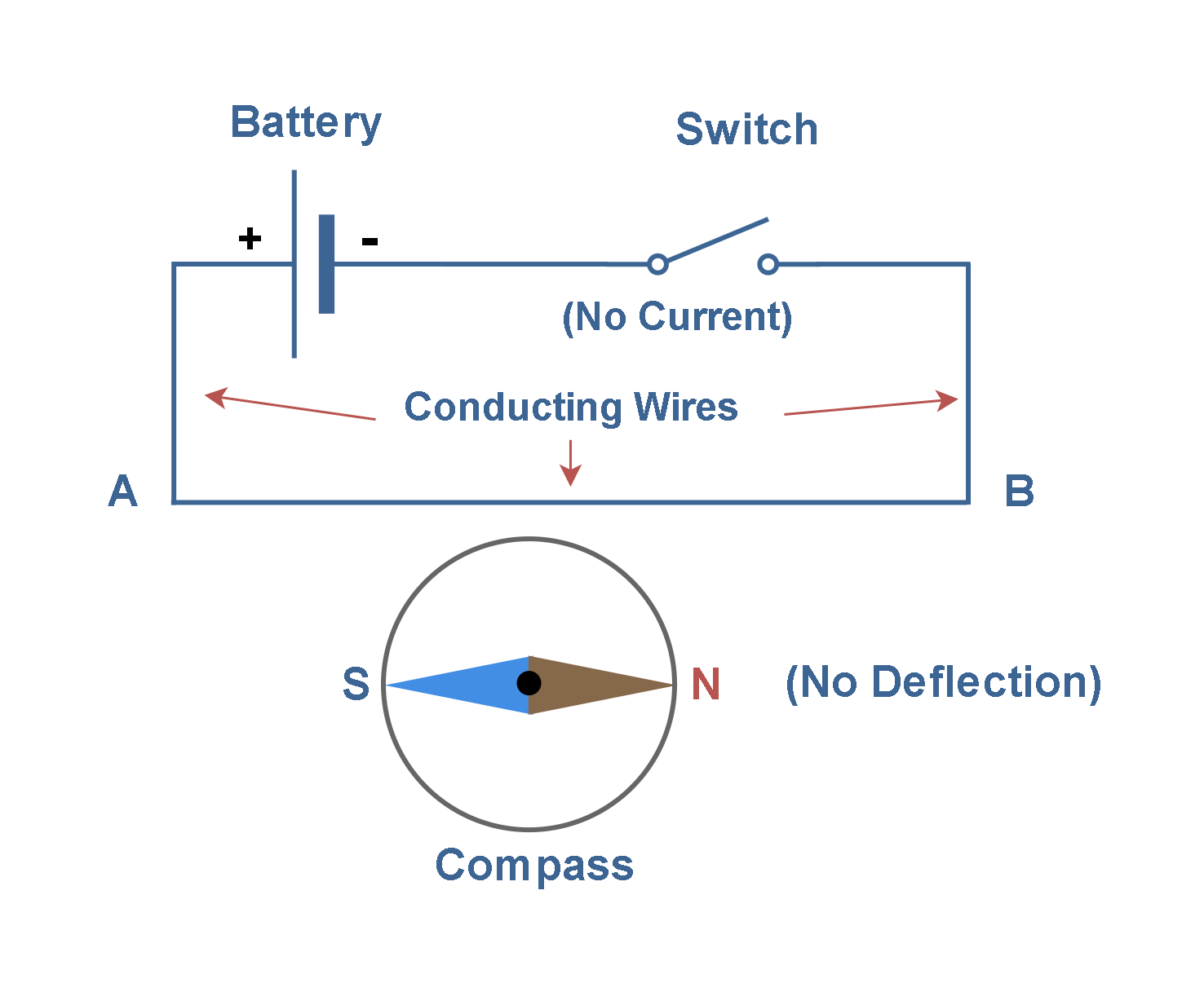
When discussing historical discoveries in magnetism, we mentioned Oersted’s finding that a wire carrying an electrical current caused a nearby compass to deflect. A connection was established that electrical currents produce magnetic fields.

Figure 1 shows a configuration of a battery, a switch, and conducting wires, which simulates Oersted’s experiment. In Figure 1a, the switch is open, so there is no current in the circuit, and the compass needle is in its natural position (pointing to the magnetic north of Earth’s sphere).

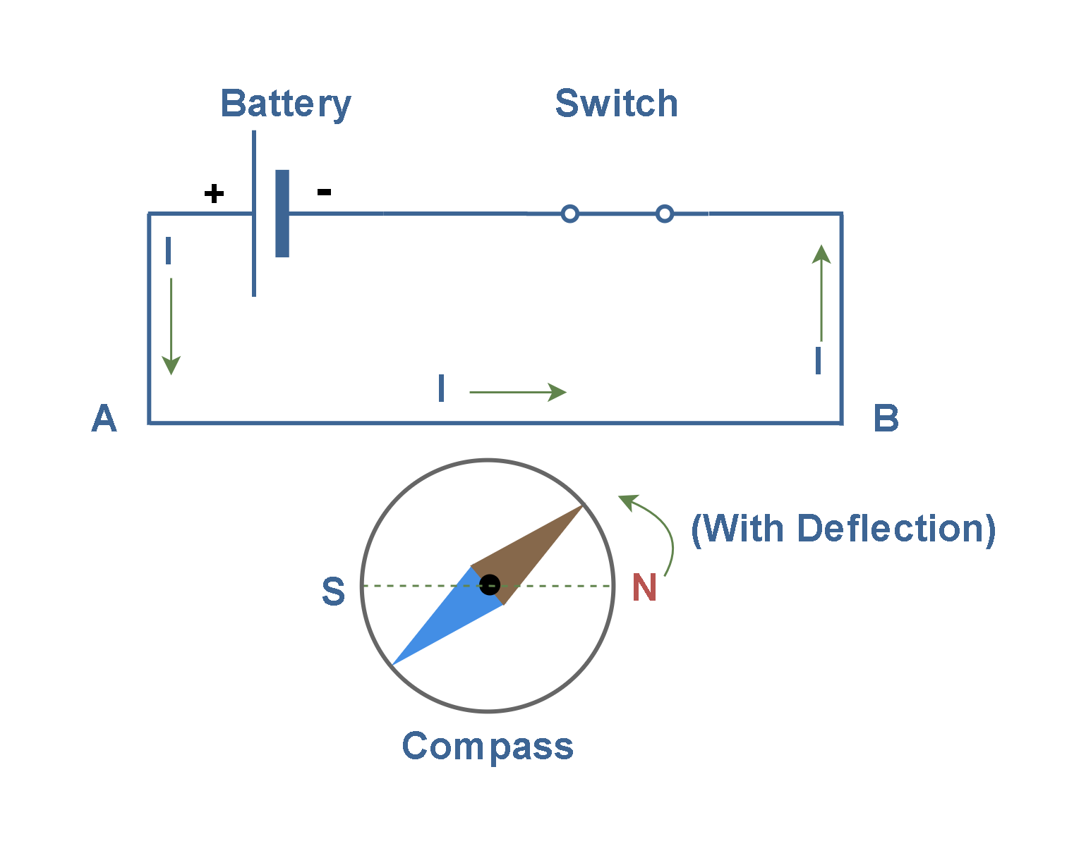
In Figure 1b, the switch is closed, so the current ‘I’ flows in the circuit and the compass needle has a deflection to the direction of west.

In Figure 1c, the polarity of the battery has been reversed, and then the current ‘I’ flows in the opposite direction, and therefore the compass needle has a deflection to the opposite direction (east).

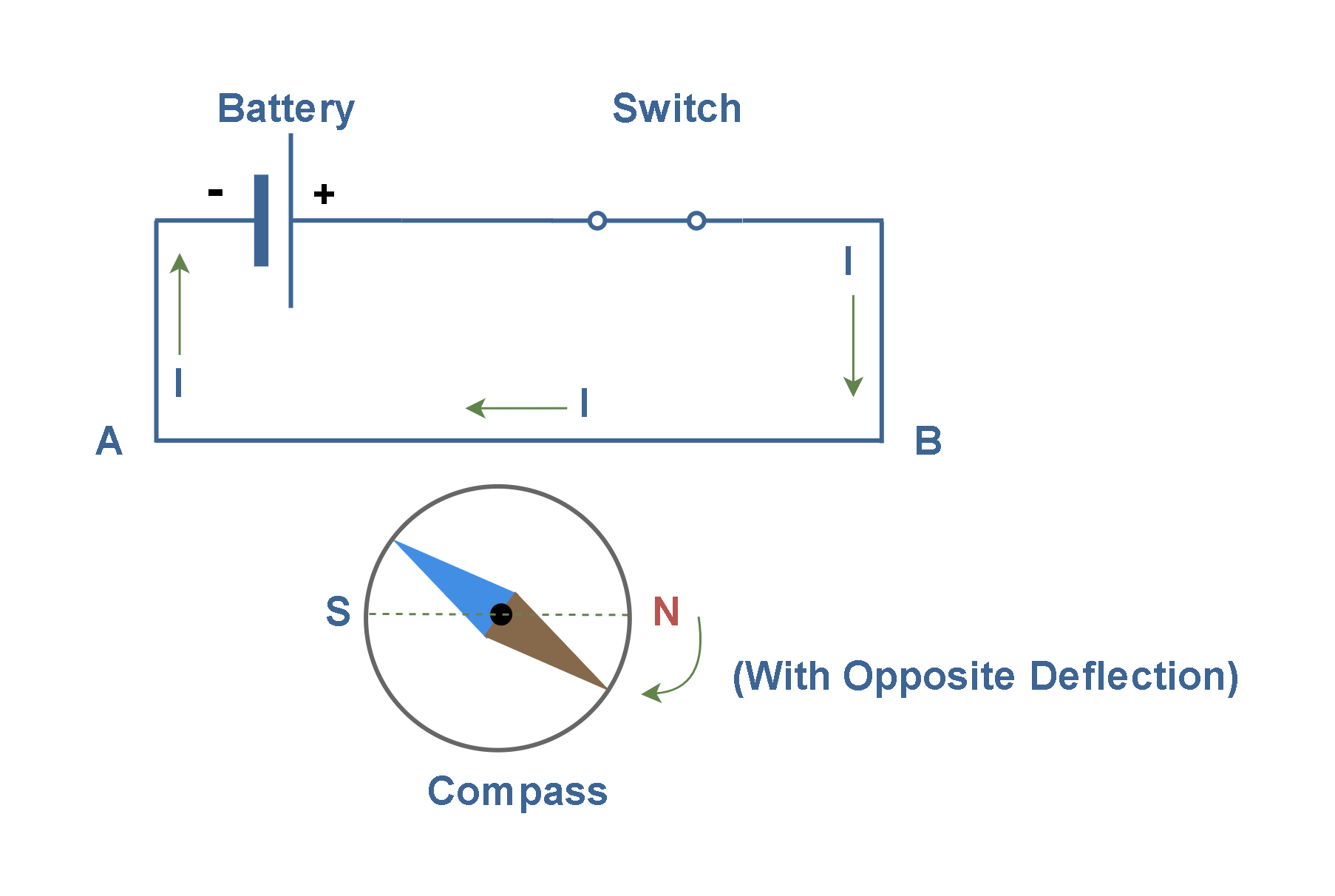
Indeed, the compass needle near the wire experiences a force which is called the magnetic force.

It was André-Marie Ampère (1775 –1836), a French physicist and mathematician, who first speculated that all magnetic effects are attributable to electric charges in motion, i.e., electric currents. Ampère also explained that a magnetized iron is full of continuously moving charges – electric currents on an atomic scale.

There are two different laws attributed to Ampere as the fundamental equations in magnetostatics: Ampere’s Circuital Law and Ampere’s Force Law. We consider them one by one.

Ampere’s Circuital Law

This law is fundamental to understanding how steady currents generate magnetic fields and is the basis for many electromagnetic applications, including inductors, transformers, and motors.

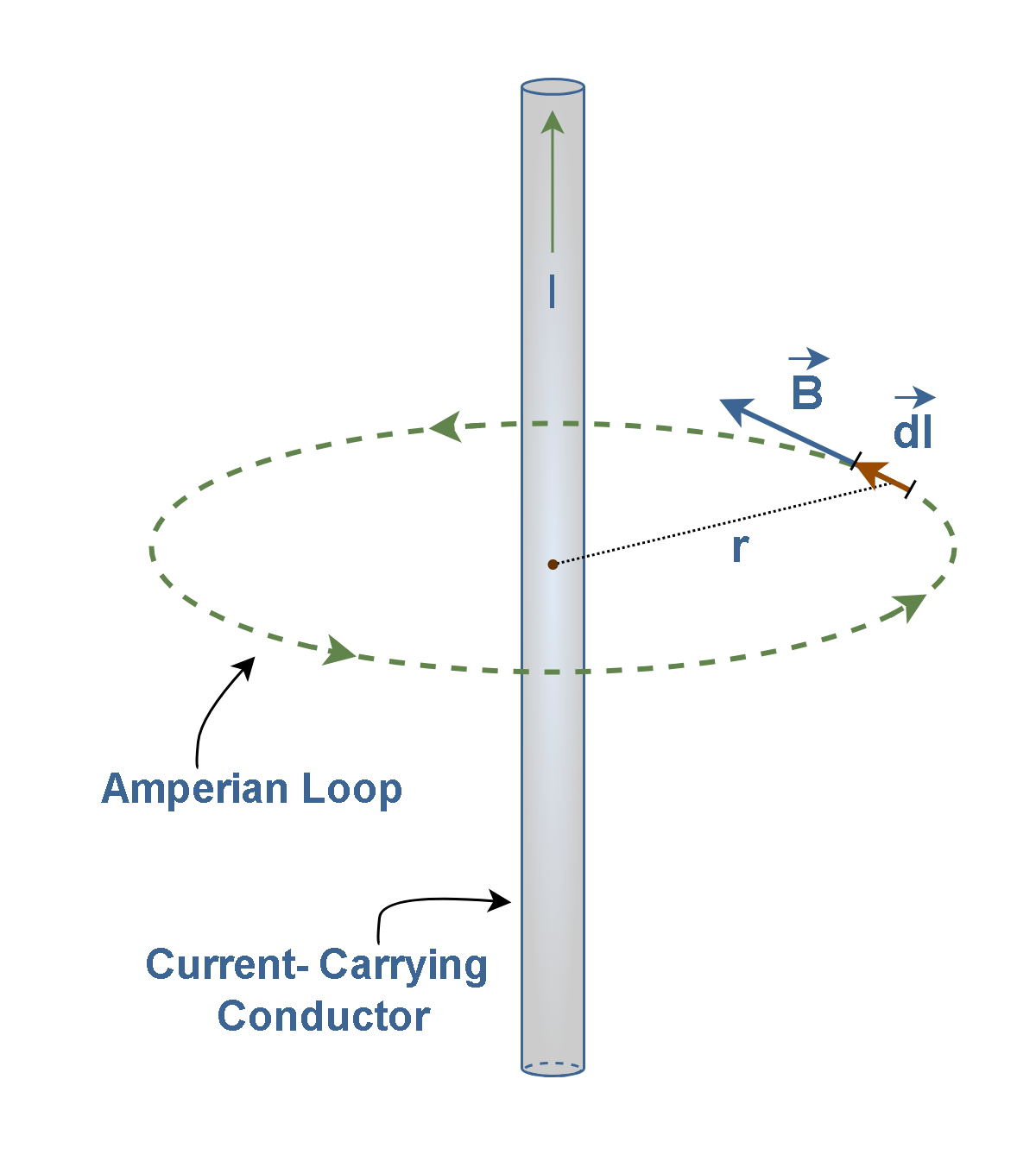
Figure 2 shows a wire carrying a steady current ‘I’ while the magnetic field vector B encircles the current tangent to a closed loop. dl is a vector whose magnitude equals an infinitesimal length of the loop, and its direction is the same as B.

The law briefly states that the integral of the magnetic field around any closed loop equals μ₀ times the current enclosed by that loop. The integral version of Ampère’s law is mathematically expressed as Equation 1:

where:

• ∮ represents the line integral around a closed loop
• B is the magnetic field vector in units of tesla (T).
• dl is an infinitesimal vector element of the loop in units of meters.
• μ₀​ is the permeability constant of free space which equals (4π × 10^-7) H/m (Henry per meter).
• I_enc​ is the total current enclosed by the loop in units of amperes.

We call I_enc the current enclosed by the Amperian loop. An Amperian loop is a hypothetical closed path used when applying Ampère’s circuital law to calculate magnetic fields. It’s a mathematical construct rather than a physical object. The green arrows in Figure 2 along the Amperian loop show the direction of integration.

The constant μ₀​ is essentially called the permeability of vacuum, and for practical purposes, it can be taken as free air, with negligible error. The permeability has much the same significance for magnetostatics as the permittivity has for electrostatics.

In particular, for currents with appropriate symmetry, Ampère’s law in integral form offers a lovely and extraordinarily efficient way of calculating the magnetic field.

If we want to use Ampere’s circuital law for different applications and structures, we should follow the next steps:

1. Identify the current distribution and its symmetry (linear, cylindrical, etc.)
2. Choose an appropriate Amperian loop that exploits the symmetry of the problem
3. Determine the enclosed current (I_enc) passing through the area bounded by the loop
4. Apply Ampère’s law by evaluating the line integral ∮ B·dl around the chosen loop
5. Solve Equation 1 for the magnetic field strength B

Let’s consider the long straight wire depicted in Figure 2. We chose a circular loop of radius r centered on the wire. B is constant and tangential to the circle circumference. Enclosed current is simply ‘I’.From vector analysis in mathematics, we remember that the dot product of 2 vectors (B . dl) results in a scalar value, which is the product of vector magnitudes and the cosine function of the angle between vectors. Here, this angle is zero, and then, the cosine equals 1.

Thus, we can simplify the calculation of Equation 1 by using just the magnitude of vectors as explained in Equation 2:

Finally, we solve Equation 2 to find the magnitude (B) as explained in Equation 3:

This result shows that the magnitude of the magnetic field B decreases inversely with distance from the wire (r).

It is important to notice that Ampère’s circuital law has some limitations. First, it is only valid for steady currents. Second, it is easiest to apply to problems with high symmetry, such as straight wires, solenoids, and toroids.

Ampere’s Force Law

This second law is what’s being referred to as “Ampere’s Force Law,” which describes the magnetic force between current-carrying conductors. Figure 3 shows a general case of two closed conducting loops (wires) C₁ and C₂ in which steady currents I₁ and I₂ flow. The current loops are assumed to be located in a vacuum.

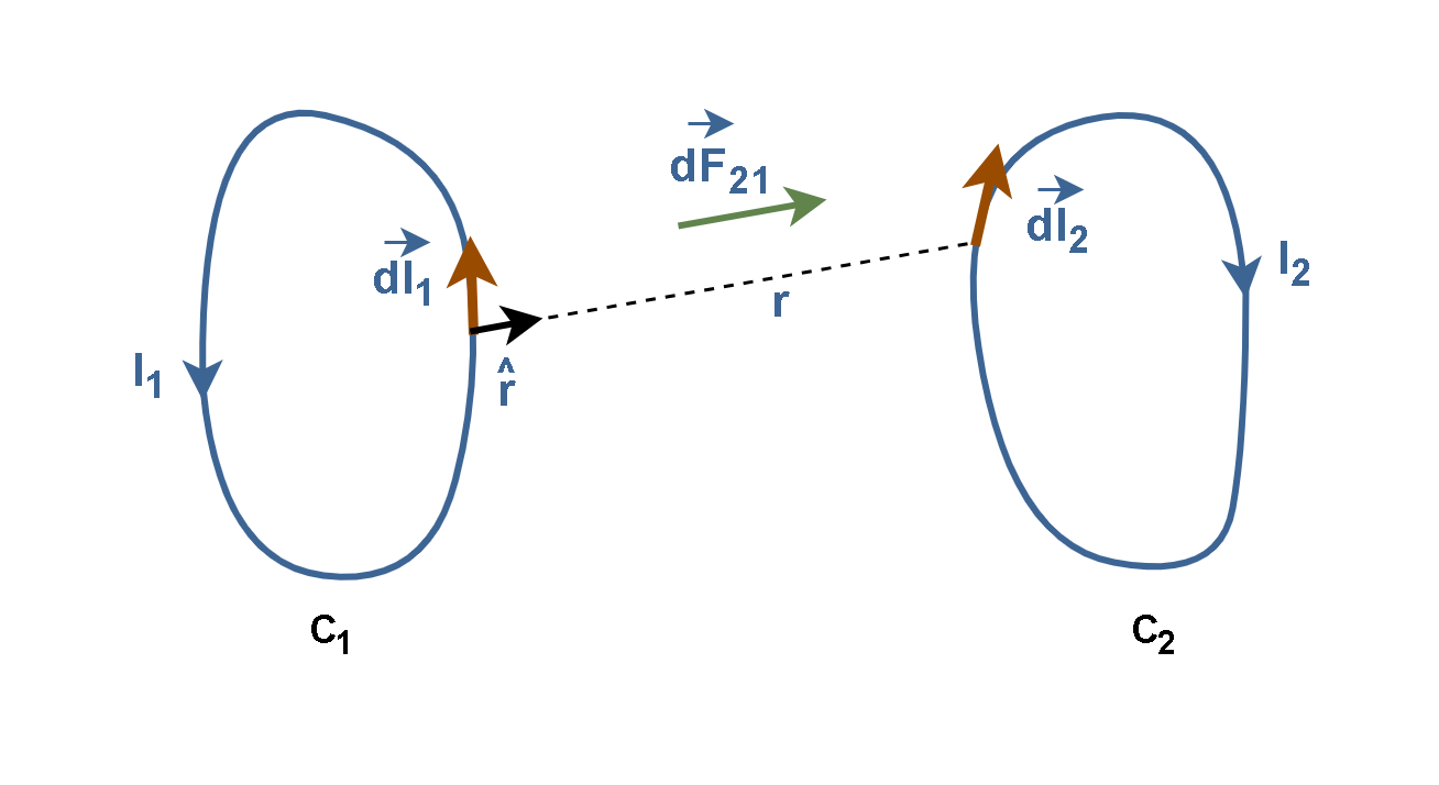
From the work of Ampere, it is found that the force element dF₂₁ exerted on C₂ by C₁ as caused by the mutual interaction of currents I₁ and I₂ may be generally expressed as Equation 4. Here, the vectorial form of force and length are considered.

where:

• dF₂₁ ​ is the differential element of force exerted on conductor 2 by conductor 1 in units of Newtons (N)
• μ₀​ is the magnetic permeability of free space (4π×10⁻⁷ H/m)
• I₁​ and I₂​ are the currents in the two conductors measured in amperes
• dl₁ and dl₂ ​ are differential elements of length along each conductor
• r^ is the unit vector pointing from the element in conductor 1 to the element in conductor 2
• r is the distance between the two elements in meters

The total force F₂₁​ can be achieved by integrating both sides of Equation 4. In its most general form, it can be defined as Equation 5:

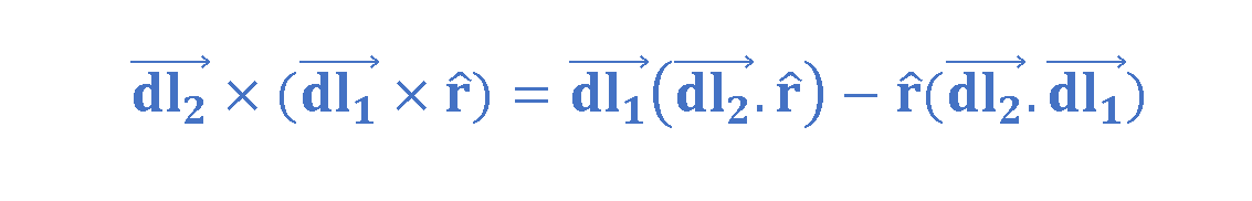
Mathematically, the double cross product in the above equations can be converted to dot-product calculations, which are simpler in computing, as explained in Equation 6:

This vectorial formulation in Equation 5 generalizes the force law for any configuration of current-carrying conductors. The resulting magnetic force F₂₁ has some properties:

• It is proportional to both currents
• It varies inversely with the square of the distance between conducting loops
• It depends on the orientation of the current elements through the cross products
• It results in attraction when currents flow in the same direction
• It results in repulsion when currents flow in opposite directions

Magnetic Forces Between Two Parallel Current-Carrying Wires

Figure 4 shows two wires, connected to two circuits (C₁, C₂), placed parallel and carrying steady electric currents (I₁, I₂) in the opposite direction. A current-carrying wire generates a magnetic field, and the magnetic field exerts a force (F₂₁ or F₁₂) on the other current-carrying wire.

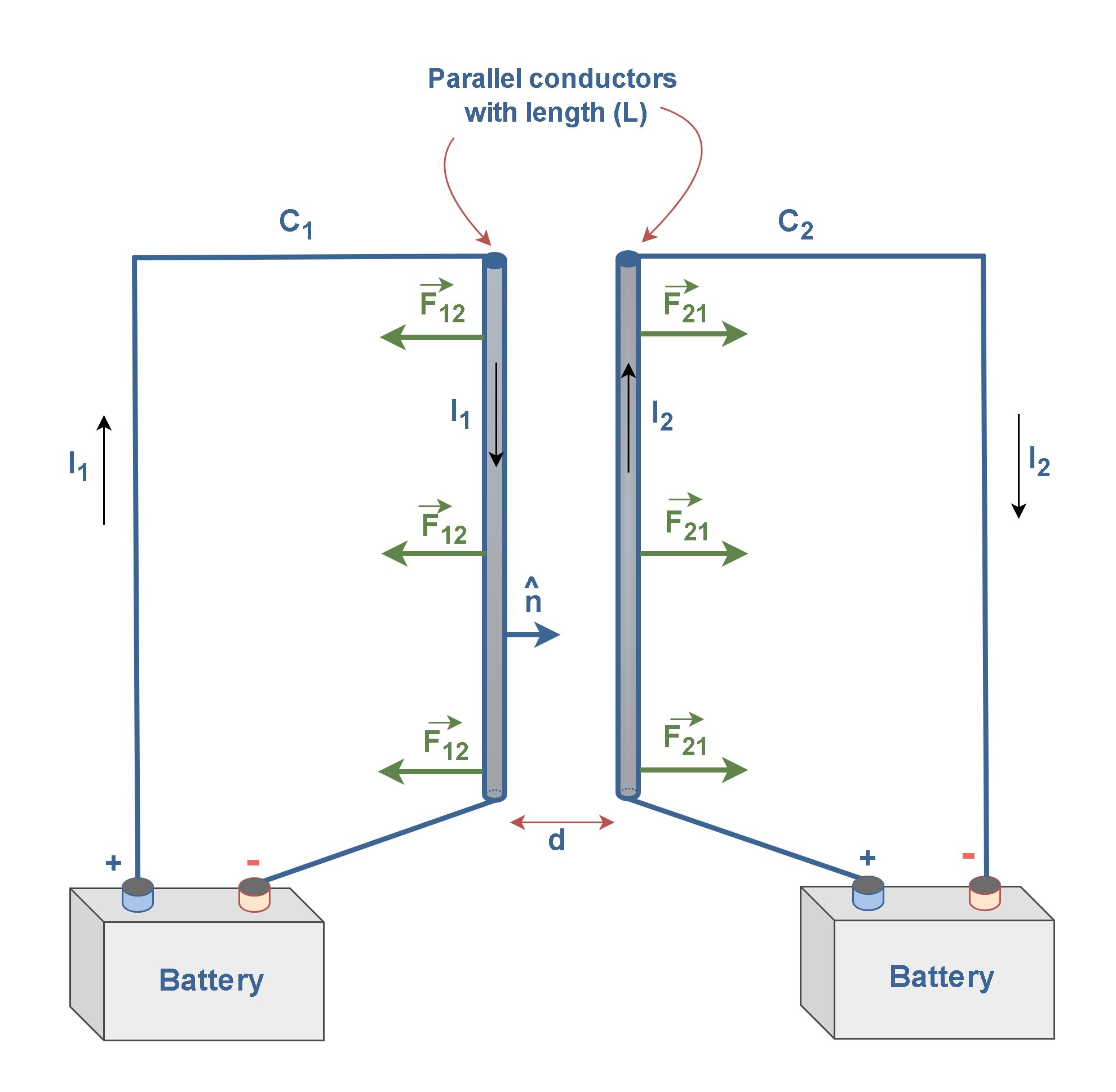
So, there is some actions at a distance as some sort of repelling force between the two wires of current. Thus, the two sections of wire in Figure 4, which are part of a circuit, tend to fly apart. Essentially, the force depends only on the charge movement in the wires, i.e., on the two currents. Reversing the direction of one of the currents changes the force to one of absorption.

For such a special case of two straight parallel conductors of length L, separated by distance d, the magnetic force can be simplified to Equation 7:

where:

• F₂₁​ is the total force on conductor 2 due to conductor 1
• F₁₂​ is the total force on conductor 1 due to conductor 2
• n^ is the unit vector pointing from conductor 1 to conductor 2, perpendicular to both conductors

Equation 7 clearly shows that the force (absorbing or repulsive) on one of the wires, per unit length of wire, is inversely proportional to the distance between the wires (d). Just in this special case, F₂₁ equals F₁₂.

This Ampere’s law of force was historically significant because it allowed the definition of the ampere as a unit of current: one ampere is the current that, if maintained in two straight parallel conductors of infinite length and negligible cross-section placed one meter apart in vacuum, would produce a force of 2×10⁻⁷ newtons per meter of length.

Summary

• The theory of steady currents is called magnetostatics.
• A static magnetic field is a magnetic field that remains constant (both in magnitude and direction) over time.
• Steady current means a continuous flow that has been going on forever, without change.
• A steady electric current always generates a magnetic field around it, as described by Ampère’s circuital law.
• Ampere’s circuital law states that the circulation of the magnetic field around a closed loop is proportional to the total current enclosed within the loop.
• Ampere’s force law describes the magnetic force between two current-carrying conductors.
• It states that two parallel conductors carrying currents in the same direction attract each other, while conductors with opposite currents repel each other.

Please follow and like us: