The Fourier Analysis – Discrete Fourier Transform (DFT)
Introduction Essentially, signals are functions that can be classified into different categories. A signal can be either continuous or discrete, and it can be either periodic or non-periodic.
Introduction
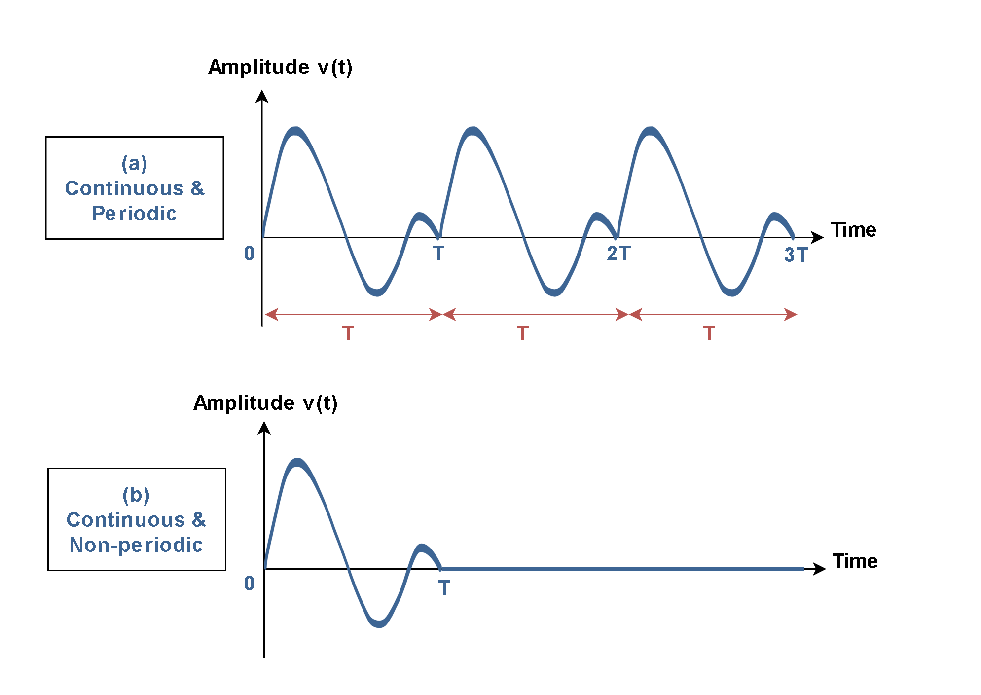
Essentially, signals are functions that can be classified into different categories. A signal can be either continuous or discrete, and it can be either periodic or non-periodic. In our ‘Analog to digital conversion’ series of articles, we have seen that it is always possible to apply a sample-and-hold circuit to an analog (continuous) signal v(t) and convert it to a new sampled (discrete) signal v[n], as shown in Figure 1 (c – d).
In this discrete signal, the amplitudes are preserved similarly to the original signal v(t), but they are defined in a number of time instances. The Sampling Theory states that the frequency of sampling (fs) should obey Nyquist’s rule. Then, the spectrum of the original signal can be preserved in the discrete signal spectra and therefore, the original continuous signal v(t) can be completely reconstructed again in the time domain from its frequency domain components.
Transforms are only different representations of the same information. The Fourier transform family allows a time domain signal to be converted into its equivalent representation in the frequency domain. Conversely, if the frequency response of a signal is known, the inverse Fourier transform allows the corresponding time domain signal to be determined.
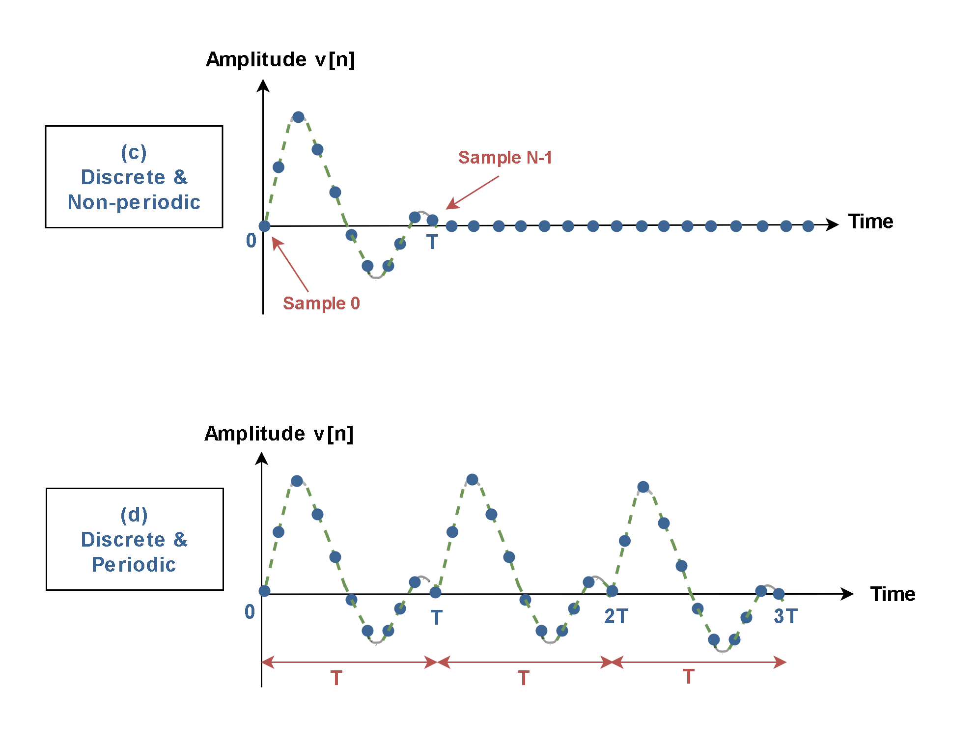
We may categorize signals based on ‘Fourier Analysis’ methods in four categories, as shown in Figure 1 (a to d):
- Continuous & Periodic: like sine waves, square waves, and any waveform that repeats itself in a regular pattern in time. The method of the Fourier transform that can be applied to these types of signals is called the Fourier Series.
- Continuous & Non-periodic: These signals are not repetitional in a periodic pattern. The Fourier method for this type of signal is simply called the Fourier Transform.
- Discrete & Non-periodic: These signals are only defined at discrete points (samples) and do not repeat themselves in a periodic fashion. This type of Fourier transform is called the Discrete-Time Fourier Transform (DTFT).
- Discrete & Periodic: These are discrete signals that repeat themselves in a periodic fashion in time. This class of Fourier Transform is called the Discrete Fourier Transform (DFT).
These four classes of real signals can be mathematically supposed to extend to positive and negative infinity in time. When we struggle with theoretical issues, we may use the first three members of the Fourier transform family (a to c). But, digital processing systems, like digital computers, can only work with information that is discrete and finite in length.
In reality, the only member of this family that is relevant to digital signal processing is the Discrete Fourier Transform (DFT). This type of transform operates on sampled time-domain signals which are periodic, as shown in Figure 1 (d).
Sometimes signals of general formats cannot be described mathematically and they also might not have periodicity, like a human’s voice signal. For such signals, the Discrete Fourier Transform (DFT) is one possible numerical approach for approximately calculating their spectrum.
Discrete Fourier Transform (DFT) Method
As shown in Figure 2, the discrete Fourier transform changes an N–sample input signal x[n] into an N-point output signal X[k]. Generally, the input and output of the DFT block can be 2 arrays of numbers that represent amplitudes. Figure 2 describes the DFT numerical method structure.
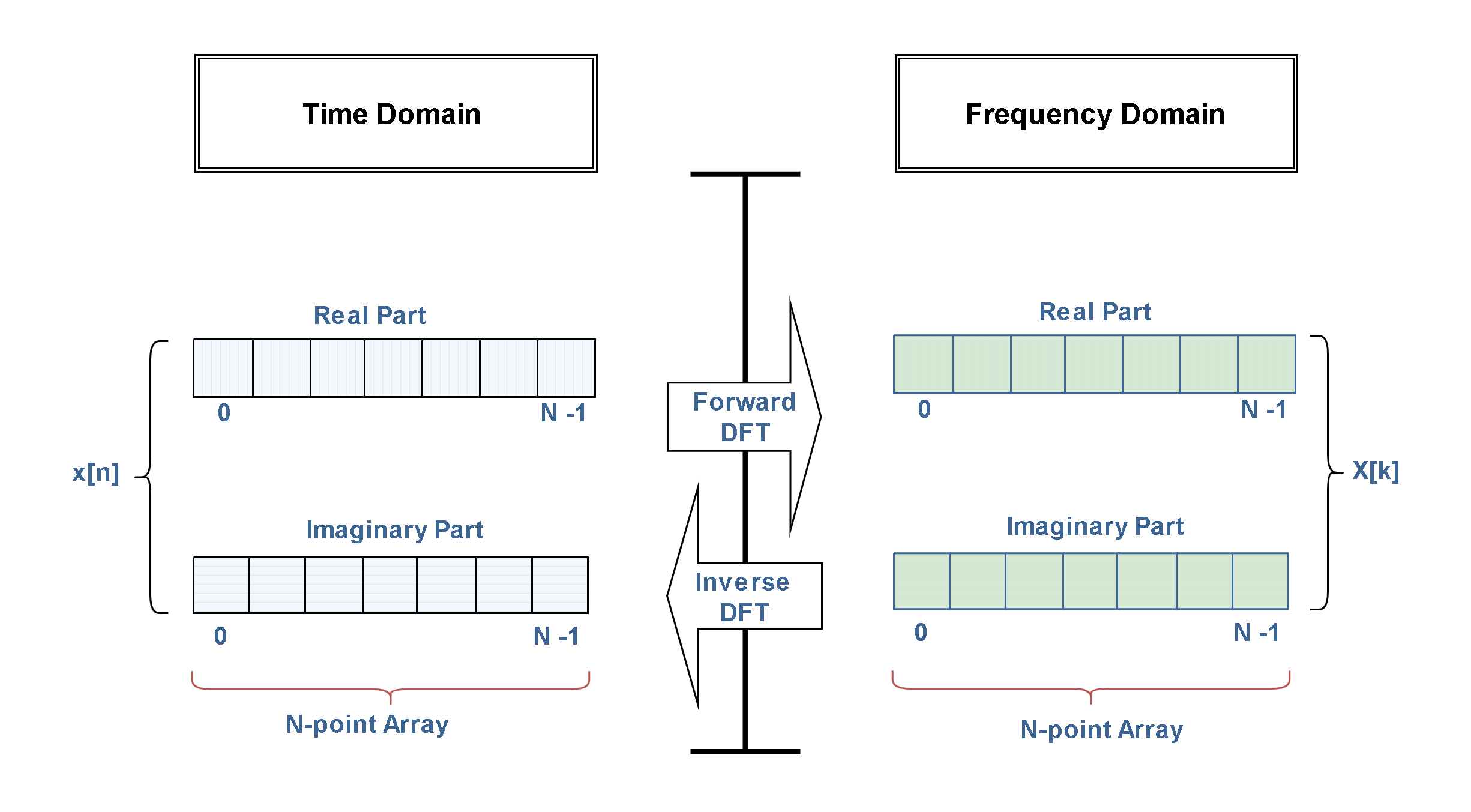
In the time domain, x[n] (lower case letter x) consists of 2 arrays of N samples as the real part (Re x[n]) and the imaginary part (Im x[n]). In the frequency domain, the DFT also produces X[k] (capital letter X) which contains two signals as the real part (Re X[k]) and the imaginary part (Im X[k]). ‘n’ is the index of samples in the time domain and ‘k’ is the index of frequency components.
Each of these signals is N points long and runs from 0 to N-1. The Forward DFT transforms from the time domain to the frequency domain, while the Inverse DFT transforms from the frequency domain to the time domain. Given the time domain signal x[n], the process of calculating the frequency domain spectrum X[n] by the forward DFT is called decomposition or analysis. If the frequency domain is known, the calculation of the time domain by the inverse DFT is called synthesis. Both synthesis and analysis can be represented in equation forms and computer algorithms.
Calculating The Complex Discrete Fourier Transform (DFT)
In comparison of DFT to continuous Fourier Transform computation, instead of an integral from minus infinity to plus infinity, only a summation formula has to be solved and this can even be done purely numerically using digital signal processing (DSP) techniques.
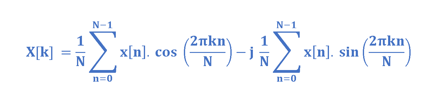
The forward complex DFT, written in polar form, is given by Equation 1.
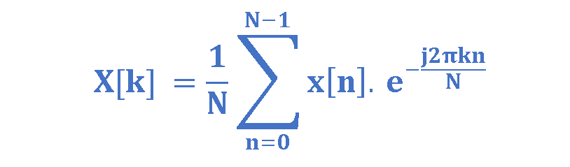
The quantity x[n] represents the nth time sample, where ‘n’ also ranges from 0 to N – 1. In Equation 1, X[k] represents the DFT frequency output at the kth spectral point, where k ranges also from 0 to N–1. The quantity N represents the number of sample points in the DFT data record. The ‘j’ is the square root of (-1) and it is an imaginary unit denoted also by √-1.
Equation 1 is in polar form, the most common for DSP. Alternatively, Euler’s relation can be used to rewrite the forward transform in rectangular form in Equation 2.
Thus, the two signals in the frequency domain which are called the real part and the imaginary part, represent the amplitudes of the cosine waves and sine waves, respectively. In spite of their names, all of the values in these arrays are just ordinary numbers. (The j’s are not included in the array values; they are a part of the mathematics of complex numbers).
However, there is scaling required to make the reconstructed signal be identical to the original signal. For the complex discrete Fourier transform, a normalization factor of 1/N must be introduced somewhere along the way.
The inverse complex DFT reconstructs the time domain signal. The inverse complex DFT, written in polar form, is given by Equation 3.
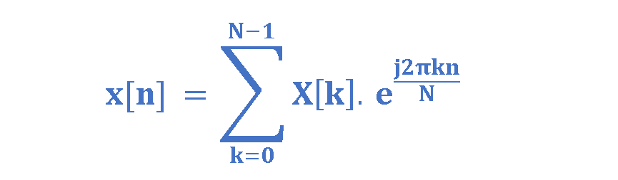
The Discrete Fourier Transform (DFT) and the Inverse Discrete Fourier Transform (IDFT) are obtained through the mathematical relations in Equations 1 and 3. These are the matching equations to transform the signals from one domain to another one.
Figure 3 shows a simple example of DFT with N = 8. First, the acquired samples of the input signal are arranged in Table 1, and then, DFT coefficients are calculated as complex numbers and collected in Table 1.
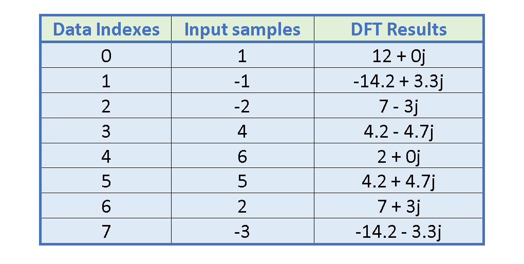
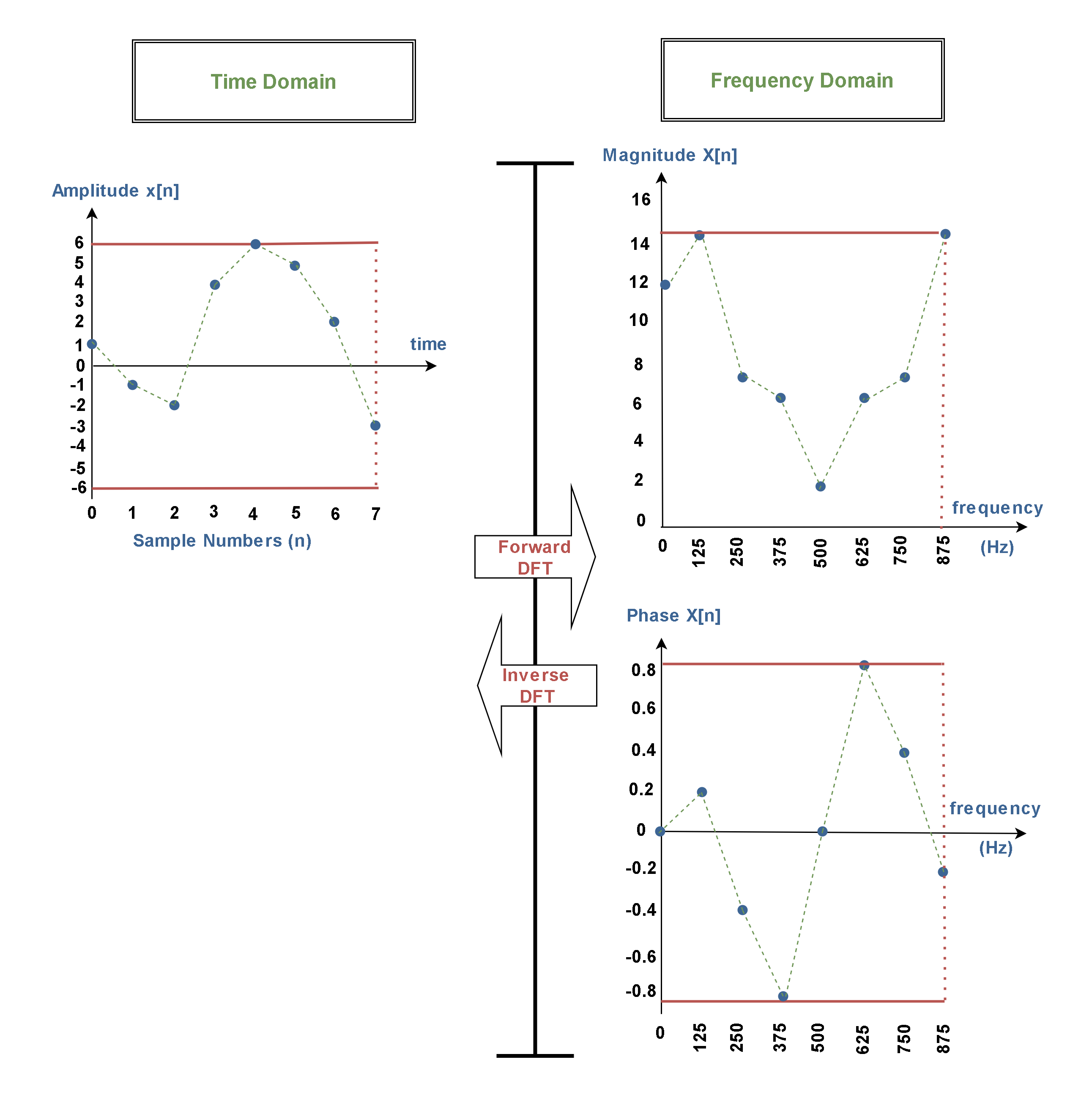
Finally, all the data are plotted in Figure 3. The time domain signal is a real signal (the imaginary part of the signal is zero) and it is contained in the array with data indexes of x[0] to x[7]. Notice that 8 points in the time domain corresponds to 8 points in each of the frequency domain signals, with the frequency indexes also running from 0 to 7.
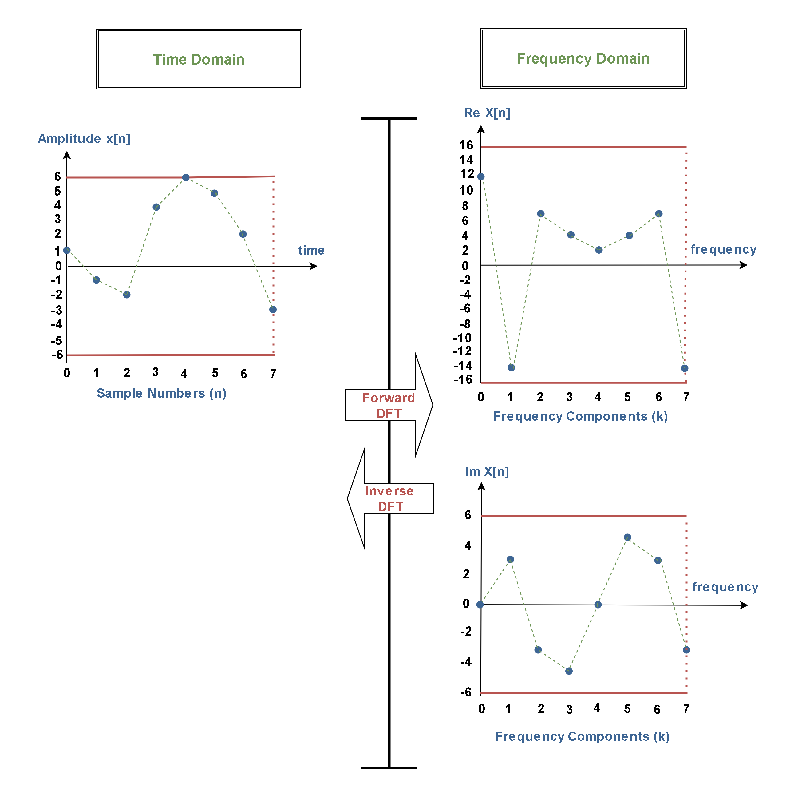
The horizontal axis of the frequency domain can be referred to in different ways. In the first method, the horizontal axis is labeled based on the spectral index (k) and corresponding to samples in the arrays. The value of k represents the position of the frequency component in the DFT output, with k = 0 corresponding to the DC component (0 Hz) and higher values of k corresponding to increasing frequencies. When this labeling is used, the index for the frequency domain is an integer from 0 to N-1. This notation is used in Figure 3.
In the second method, the horizontal axis is labeled as frequency in terms of Hertz. In this case, we need to know the sampling rate (fs) of the input signal. The index used with this notation is f, for frequency. To convert from the first notation, k, to the second notation, f, we can use Equation 4.

Then by assuming fs = 1000 Hz in our example we can rewrite the results and plot them in Figure 4.
Also, for better understanding, it is possible to plot the results based on ‘Magnitude’ and ‘Phase angle’ instead of the real and imaginary parts in the frequency domain. For this reason, we can use Equation 5 to calculate the magnitude of the transformed coefficients which are in the complex form (z = a +jb).

It is also possible to use Equation 6 for finding the phase angle of transformed coefficients.

The results of the calculation are written in Table 2.
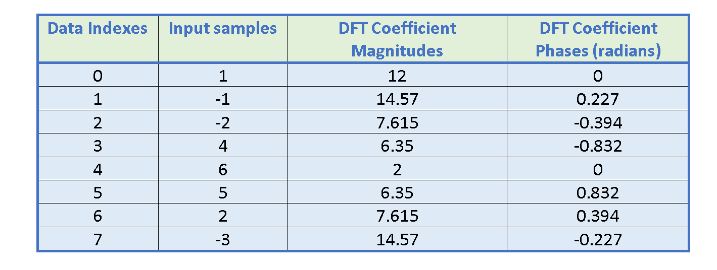
Figure 4 shows the complex frequency spectrum plot resulting from the DFT calculation in terms of the magnitude and the phase with (N =8) and (fs = 1000 Hz).
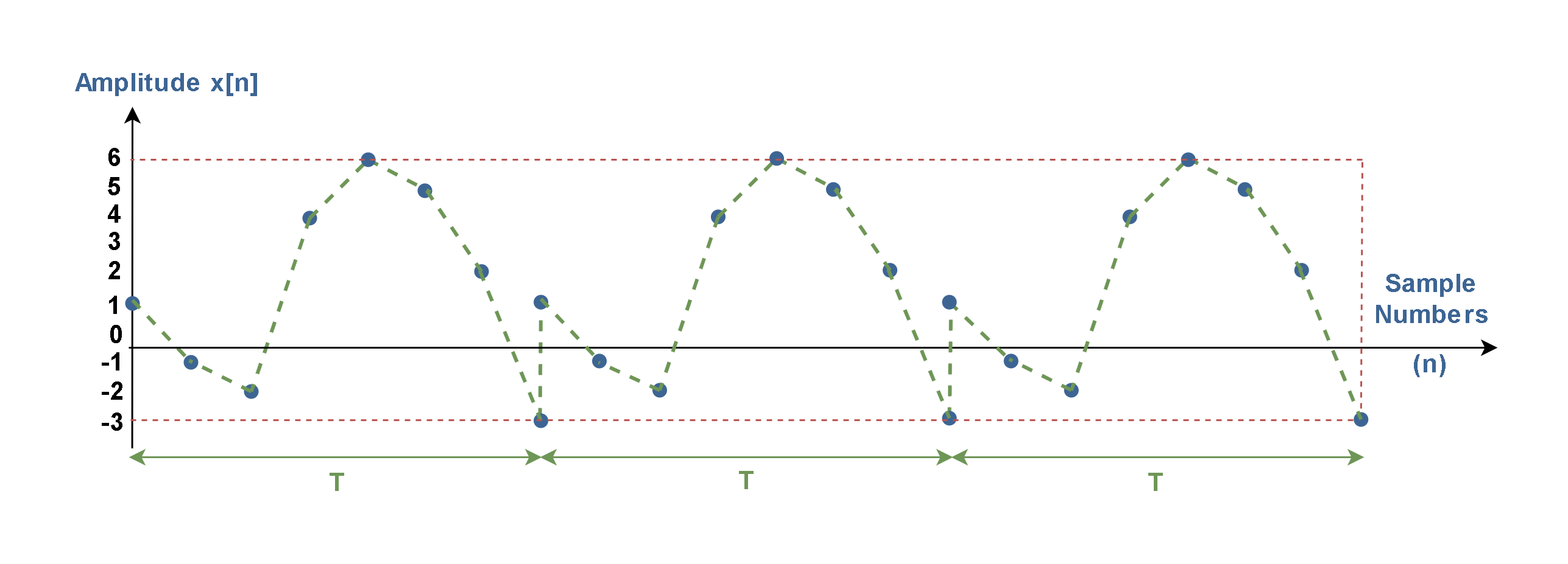
Essentially, the DFT views these N points to be a single period of an infinitely long periodic signal. When we calculate the DFT of a periodic time-domain signal, as explained in Equation 7, the resulting DFT coefficients also exhibit periodicity, as explained in Equation 8. It means, the DFT coefficients repeat or oscillate every N coefficient.


However, in the real world, only a finite number of samples (N) are available for input into the DFT. This problem is overcome by placing an infinite number of groups of the same N samples “end-to-end”. This means that the left side of the acquired signal is connected to the right side of a duplicate signal. Likewise, the right side of the acquired signal is connected to the left side of an identical period.
This technique constructs a periodic sequence by repeating the real N-sample sequence and forces mathematical (not real-world) periodicity. Figure 5 shows this periodicity in the time domain.
Periodicity in the frequency domain behaves in much the same way but is more complicated. The complex Fourier transform includes both positive and negative frequencies. Taking these negative frequencies into account, the DFT views the frequency domain as periodic.
The Discrete Fourier Transform (DFT) actually corresponds to a Fourier analysis within the window of observation (N samples) of the signal. It is thus assumed that the signal in the observed time window continues periodically. This assumption results in “uncertainties” in the analysis so that the Discrete Fourier Transform can only supply approximate information about the actual frequency band.
Advantages of DFT
The Discrete Fourier Transform is a fundamental mathematical tool used in various fields, including audio processing, image analysis, speech recognition, data compression, and many types of measuring equipment. It is widely employed for analyzing and manipulating signals in both the time and frequency domains.
In general, we need the Fourier transform if we need to look at the frequencies in a signal. Signals and waveforms in electronics and communication applications are expressed by using both time-domain and frequency-domain plots, but in many cases, the frequency-domain plot is more useful.
Fourier analysis allows us to determine not only the frequency components in any sophisticated signal to make its spectrum but also how much bandwidth the particular signal occupies. Although a sine or cosine wave at a single frequency theoretically occupies no bandwidth (with single-line spectrums), sophisticated signals obviously take up more spectrum space. For example, a 1-MHz square wave with harmonics up to the eleventh occupies a bandwidth of 11 MHz!
Real-time spectrum analyzers are indeed common applications of the DFT. These instruments use DSP processors that are programmed to perform DFT computations on incoming signals in real time. The DFT results are then used to display the frequency spectrum of the input signal in a graphical format, making them valuable tools for signal analysis and troubleshooting.
Summary
- Signals can be categorized as continuous-time and discrete-time functions, in the forms of periodic or non-periodic.
- By using an analog-to-digital converter (ADC), the signal is sampled at discrete points in the time domain and observed only within a limited time window at N points.
- We start with a time domain signal and take the DFT to find the frequency domain signal. To reverse the process, we take the Inverse DFT of the frequency domain signal, reconstructing the original time domain signal.
- Briefly, the complex DFT transforms two N point time domain signals into two N point frequency domain signals. The two time-domain signals are called the real part and the imaginary part, just similar to the frequency-domain signals.
- Both the time domain samples, x[n], and the frequency domain data, X[k], are arrays of complex numbers, with k and n running from 0 to N-1.
- The DFT views both the time domain and the frequency domain as periodic forms.
- The DFT operates on a finite number (N) of digitized time samples, x[n]. When these samples are repeated and placed “End-to-End,” they appear periodic to the transform.
- If working with a signal in the time domain is difficult, then using the Fourier transform to move it into the frequency domain is worth trying.


