Analog To Digital Conversion – Sampling and Quantization
This article presents two key concepts in converting a continuous analog signal to a discrete digital signal. It also examines key challenges and basic system implementations.
Converting Continuous Analog Signals To Discrete Digital
By definition, an analog signal changes continuously over time, and it has an infinite variety of amplitude values as time goes on. The best example of an analog physical signal is our voice. Whatever we speak, we generate sound waves, and this sound (message) travels through waves. The main characteristics of analog signals are amplitude, frequency, and phase.
If an alternating current (AC) line voltage is viewed on a conventional oscilloscope, the display shows a continuous sine waveform. On that curve, an instantaneous amplitude value might be 100, 99.8, or 99.875 volts. Given different resolutions, there are different real numbers or possible values.
Nowadays, we live in a wide digital world of numbers, texts, and symbols, and similar discrete data, which would seem to necessitate digital circuits and systems like arithmetic and logic computing and storage systems.
Digital techniques initially began with electromechanical devices like relays. These were eventually replaced by vacuum-tube logic circuits, which were gradually followed by discrete transistors, small-scale ICs, and finally large-scale and fast microprocessors with billions of transistors. Digital methods and computational applications are currently used for almost all parts of our lives: keeping track of money, and transferring words, sounds, images, and videos.
Utilizing digital signals and systems essentially have some advantages:
- Digital signals are very easy to analyze and process
- Although digital signals can be easily stored and accessed comfortably.
- Digital systems normally produce less noise and consume less power than their analog counterparts.
The Analog-to-Digital converter has numerous applications. For example, it is used in a digital communication system (like a cellular phone) where the analog signal to be transmitted is digitized at the sending end by an A/D converter. It also forms an essential interface when it comes to analyzing analog data with a digital computer. Figure 1 shows the system diagram of the A/D converter.
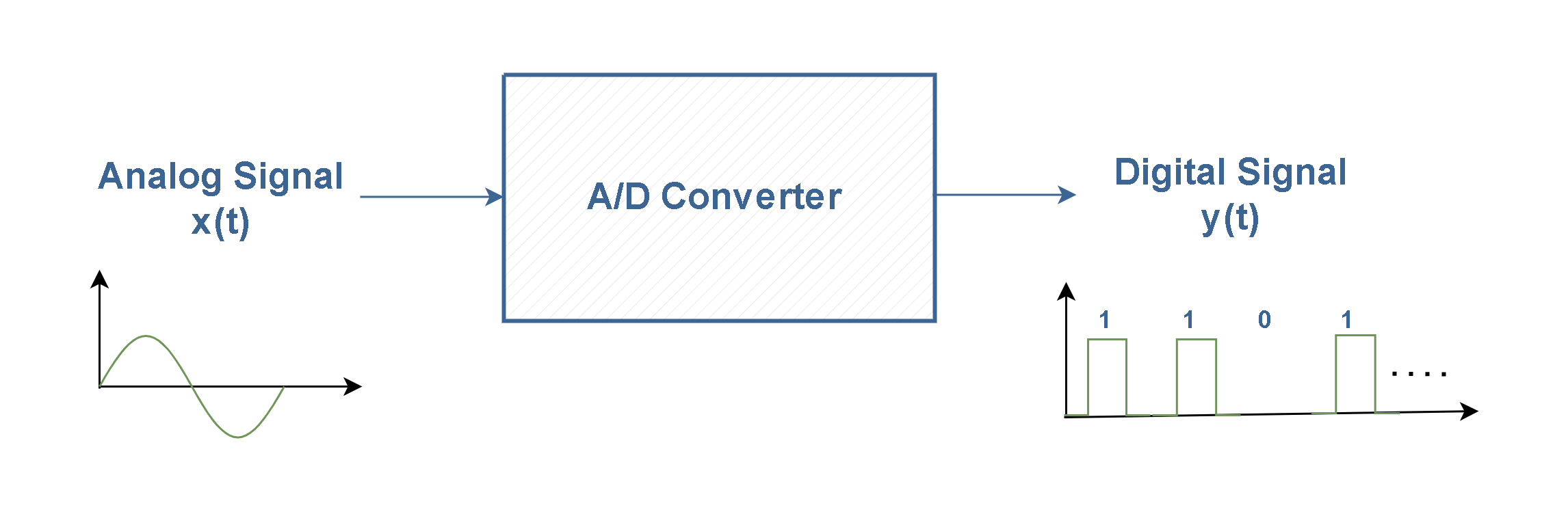
Figure 1: The A/D converter
Essentially, most of the electronic sensors (sound, image, …) are in the analog form. Therefore, the A/D converter (as a part of digital processing) is used in all digital read-out test and measuring equipment; whether in a digital multimeter or a digital storage oscilloscope or even a pH meter.
We normally expect to utilize the advantages of converting the analog signals to digital form and it is mostly supposed to recover the signals into their original forms (analog) again at the final stage. The main process is referred to as A-to-D conversion or as digitization. The reverse of this process is called D-to-A conversion which means turning the digital information back into analog form. The A/D conversion process is generally more complex than the D/A conversion process.
A/D Conversion Method
The physical nature of an A/D converter is such that it divides a voltage range into discrete values, each of which is then represented by a binary number. There are many different ways in which an analog signal may be turned into a digital form. Several different techniques have evolved for dealing with different system requirements. These include flash, staircase, successive approximation, and delta-sigma forms.
In this article, we will only consider one of the most popular methods, called Pulse Code Modulation, or PCM for short. This concept of A/D conversion is simple: first, the voltage of the incoming waveform is measured at specific instances in time. Then, these measurements will be quantized and finally translated into some digital words. Figure 2 shows the block diagram of a PCM system.
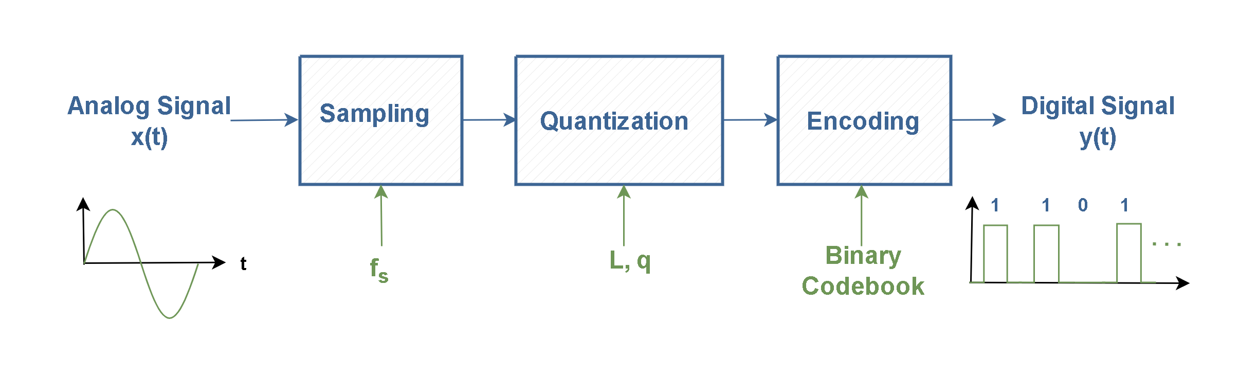
Figure 2: The PCM System
Based on the theory of PCM, to convert an analog signal into a digital form there are three functional steps:
- Sampling
- Quantization
- Digital Encoding
Sampling
The first step involves transforming the signal from continuous-time domain into discrete-time domain. This process is achieved by sampling technique. A sampler systematically extracts some amplitude values in some instants of time, like an electronic switch. It means sampling is done along the x-axis of signals.
This mechanism is shown graphically in Figure 3.
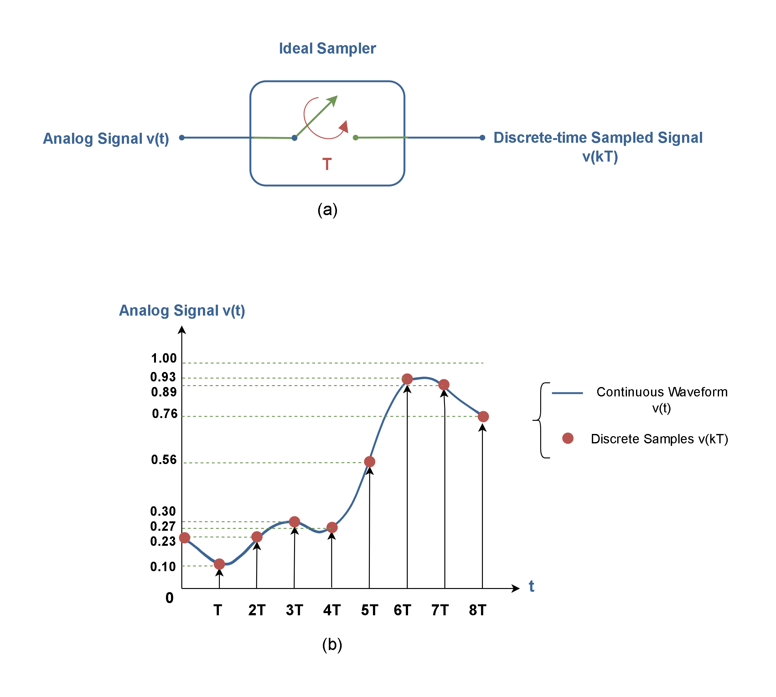
Figure 3: The Ideal sampling system (a) and (b) input/output waveforms
The result of ideal sampling is a series of impulses (or spikes) with amplitude values representing the input signal v(t) amplitude values at different instances. Figure 3 (a) shows that the analog signal is sampled by the electronic switch once every T seconds (for example every 0.5 s), resulting in a sampled amplitude sequence; which is known as a discrete-time signal. Such discrete-time signals can have any amplitude values (similar to analog signals), but at specific points in time; as shown in Figure 3 (b). At other times, the amplitudes are unknown. Briefly, such discrete-time signals are discrete in time, but still continuous in amplitude.
The sampler switch is also assumed to be ideal in which the value of the signal is taken at an instant (an infinitely small time). The time interval between samples is mostly held constant, i.e., the rate of sampling is constant. This condition is called uniform sampling.
The most important parameters in the sampling process are the sampling period T, and the sampling frequency or sampling rate which is defined as fs. The sampling frequency is given in units of ‘samples per second’ or ‘Hertz’.
The Nyquist-Shannon sampling theorem specifies the minimum sampling rate at which a continuous-time signal needs to be uniformly sampled so that the original signal can be completely recovered (or reconstructed) again by these samples alone. This rate is called the Nyquist rate.
If a continuous-time signal contains no frequency components higher than fmax (Hz), as it is represented in Figure 4 (a), then it can be completely determined by uniform samples taken at a rate fs (samples per second) whereas it is explained in Equation 1. To simplify notations, we define fmax = W.
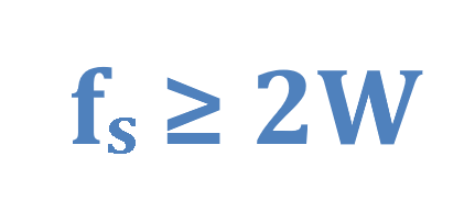
Equation 1: The sampling frequency condition
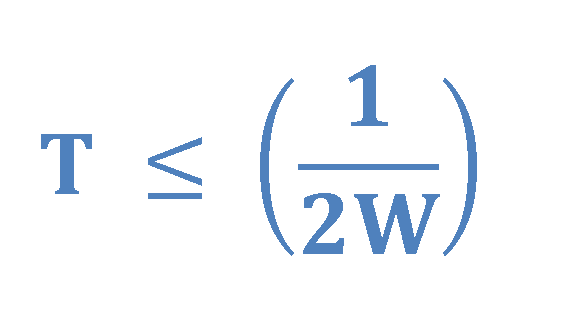
Equation 2: The sampling period condition
For example, if a signal with a bandwidth up to 20 kHz (like the sound signal) needs to be digitized, then a sample rate of at least 40 kHz is required.
A better understanding of the sampling theorem could be obtained by looking at the sampling process from the frequency domain perspective. Essentially, the sampling process is equivalent to the chopping of the original (analog) signal in the time domain. It can be shown through the Fourier transform theory that this chopping (or switching) function introduces a large number of high-frequency components into the signal spectra.
The high-frequency components generated by sampling appear in a very regular fashion. In fact, every frequency component in the original signal spectrum is periodically repeated over the entire frequency axis. Notice that spectra mathematically extend to negative frequencies also! The period at which this replication occurs is determined by the sampling rate, fs. Replication of the signal spectrum for a bandlimited signal after sampling is shown in Figure 4 (b).
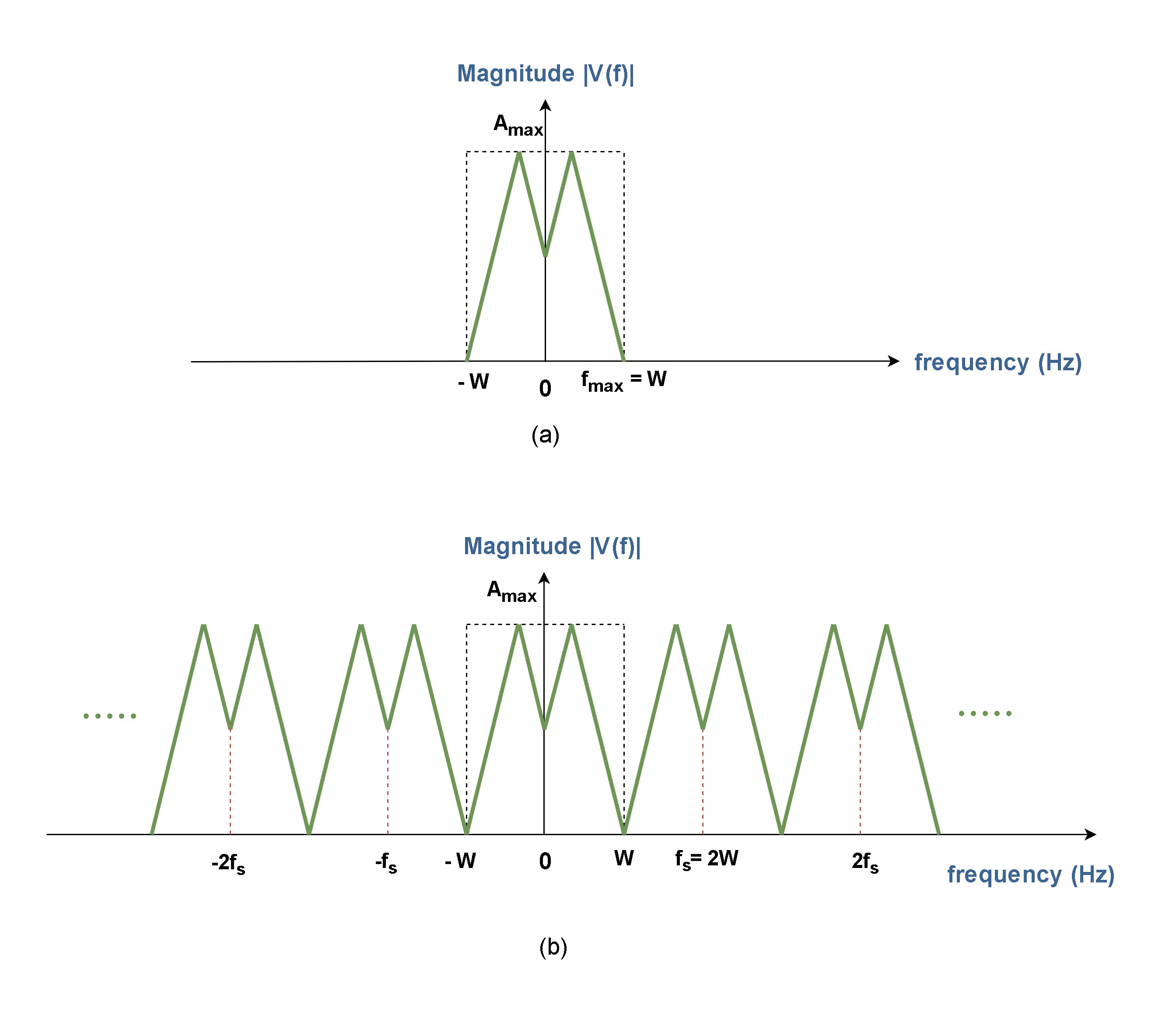
Figure 4: (a) Spectrum of the original analog signal (b) Spectra of the sampled signal
The Nyquist-Shannon sampling theorem states that if the sampling frequency is at least twice the highest frequency of the spectrum (fs = 2W), the replicated spectra do not overlap, and no distortion occurs. Thus, the original spectrum can be faithfully recovered again by suitable frequency filtering.
Consider the effect if the sampling frequency is less than twice the highest frequency component (fs < 2W). As shown in Figure 5, the replicated spectra overlap each other, causing distortion to the original spectrum. Under this circumstance, the original spectrum can never be recovered faithfully. This effect is known as aliasing.
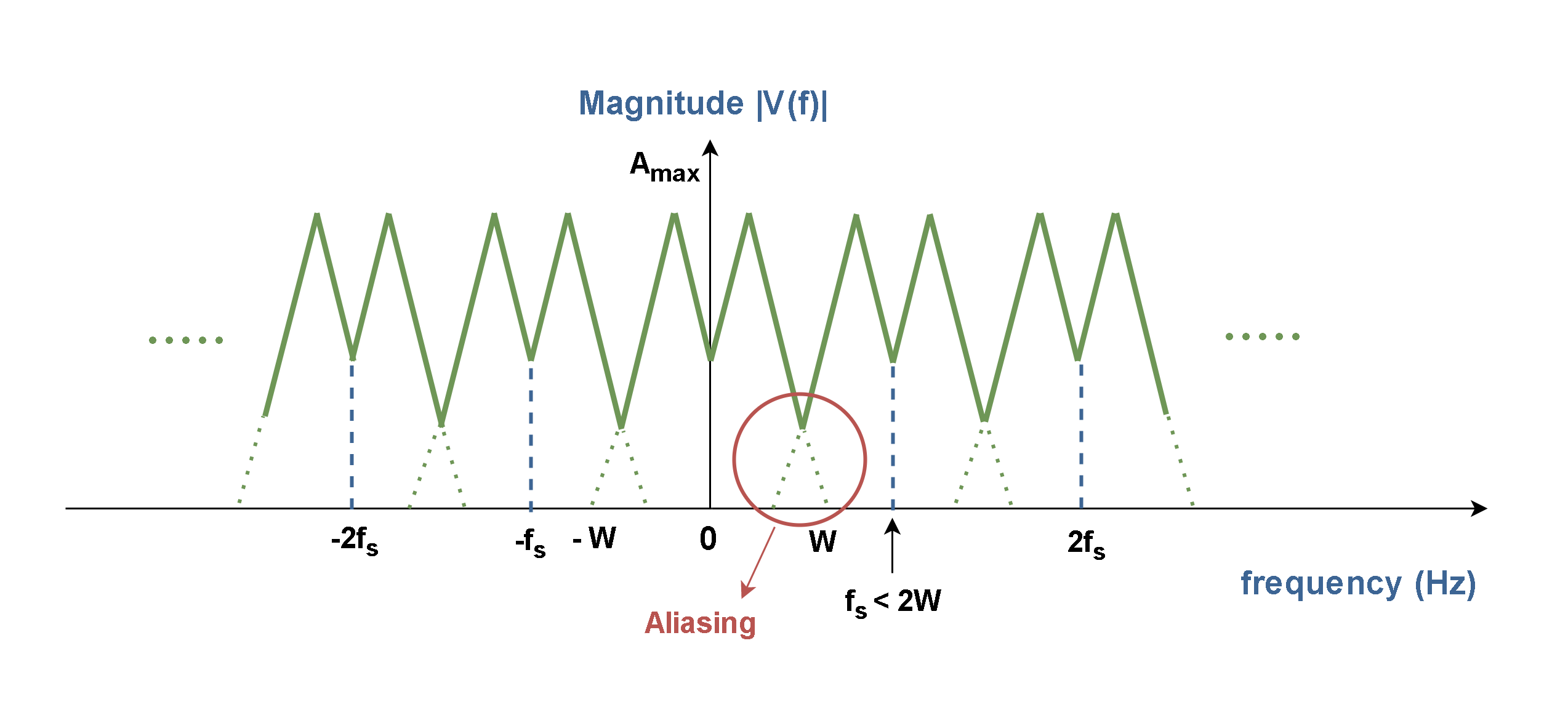
Figure 5: Aliasing distortion in frequency
The aliasing effect in the time domain is shown graphically in Figure 3-1. Normally, in a sequence with a sampling rate greater than the Nyquist rate, if we connect the sample points together by some imaginary lines, it is supposed to make a shape that is similar to the original continuous waveform. This case is shown in Figure 6 (a). But, in the case of fs < 2W the number of sample points is not sufficient to restore the original waveform. Thus, the original waveform has completely disappeared in Figure 6 (b) and this is the real meaning of the alias.
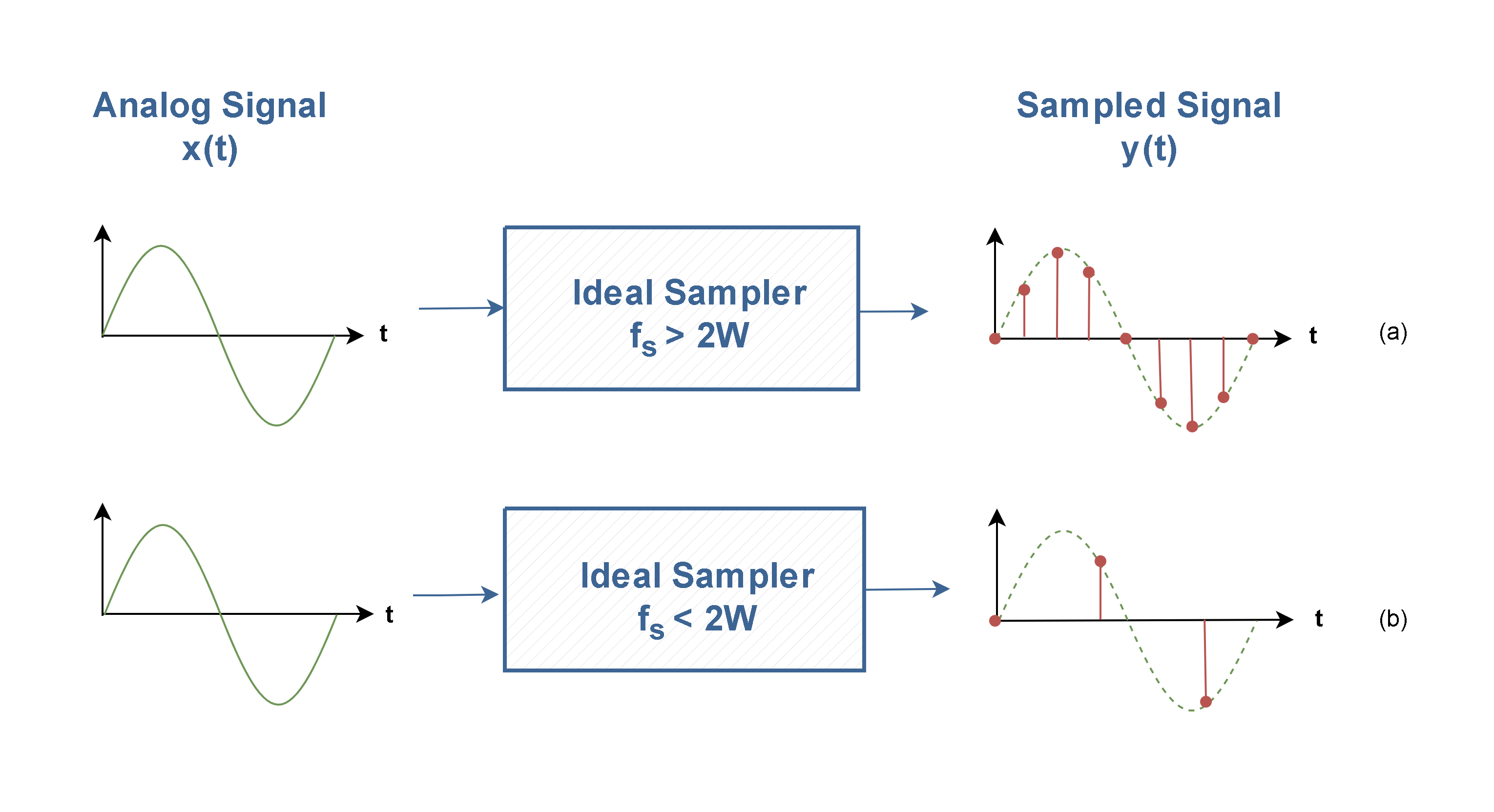
Figure 6: Aliasing distortion in time
In order to prevent the aliasing effect, the input signal must be already frequency-band limited. That is, a low-pass filter (often referred to as an anti-alias filter) must be used before A/D conversion takes place.
The low pass filter (LPF) passes signals with a frequency lower than a selected cutoff frequency (fc) and eliminates the higher frequency components present in the input analog signal to ensure that the input signal to the sampler is free from the unwanted frequency components. The ideal filter has a flat passband and a sharp cutoff behavior.
The block diagram of an ideal LPF is shown in Figure 7 (a) and its transfer function in the frequency domain is depicted in Figure 7 (b).
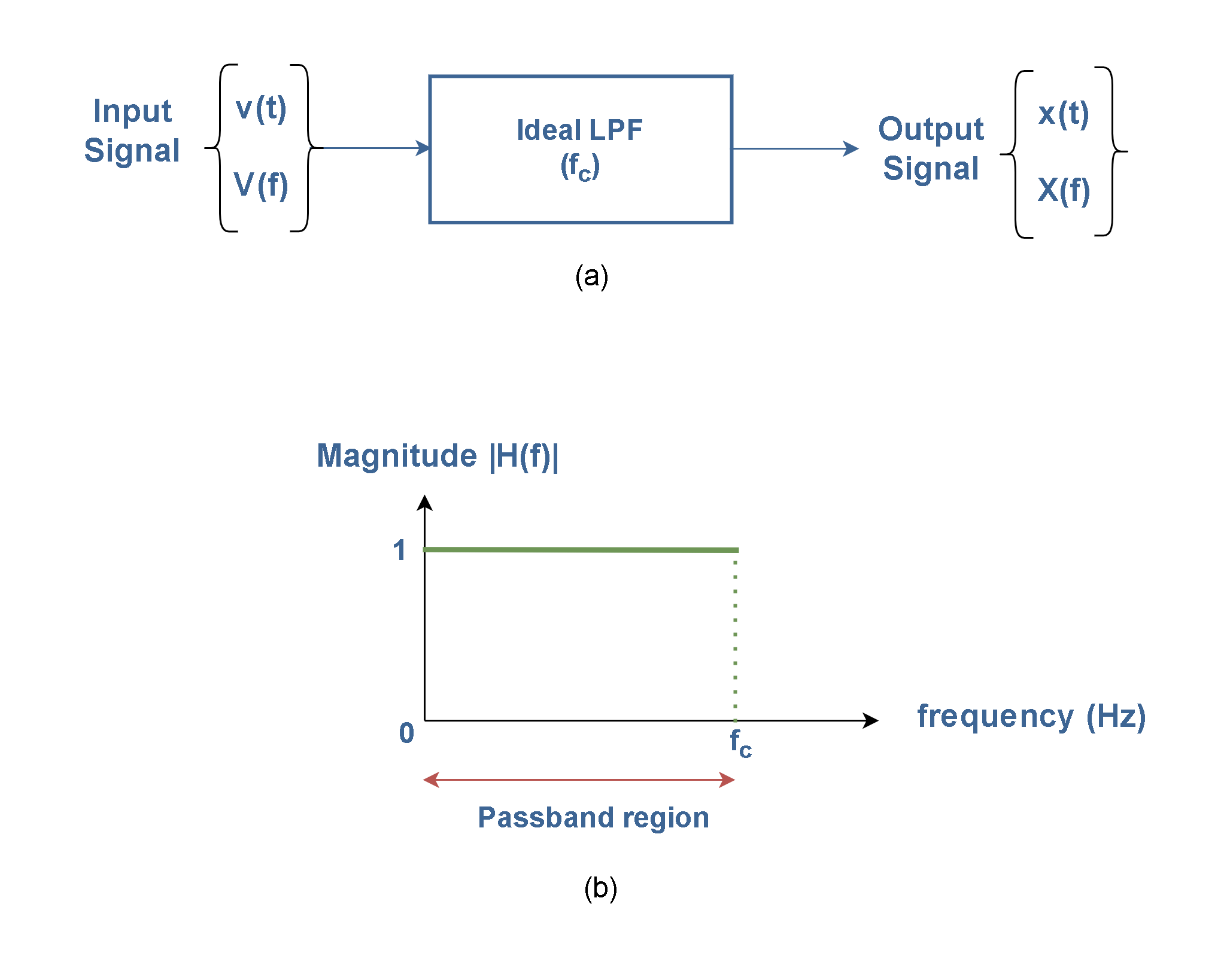
Figure 7: (a) The block diagram of an ideal LPF, and (b) the Transfer function
The sampling system incorporating an ideal low-pass filter is shown in Figure 8 (a). Assume that the spectrum of an analog signal has some frequency components more than fs/2, as shown in Figure 8 (b). If the cutoff frequency of this filter is defined as half of the sampling frequency (fc = fs/2), those portions of the spectrum with higher frequencies and small magnitudes will be eliminated by the filter. Thus, the spectrum of the signal after low-pass filtering is shown in Figure 8 (c). Mostly there is no important information in those omitted frequency components and finally, the signal can be restored again by the remained spectrum.
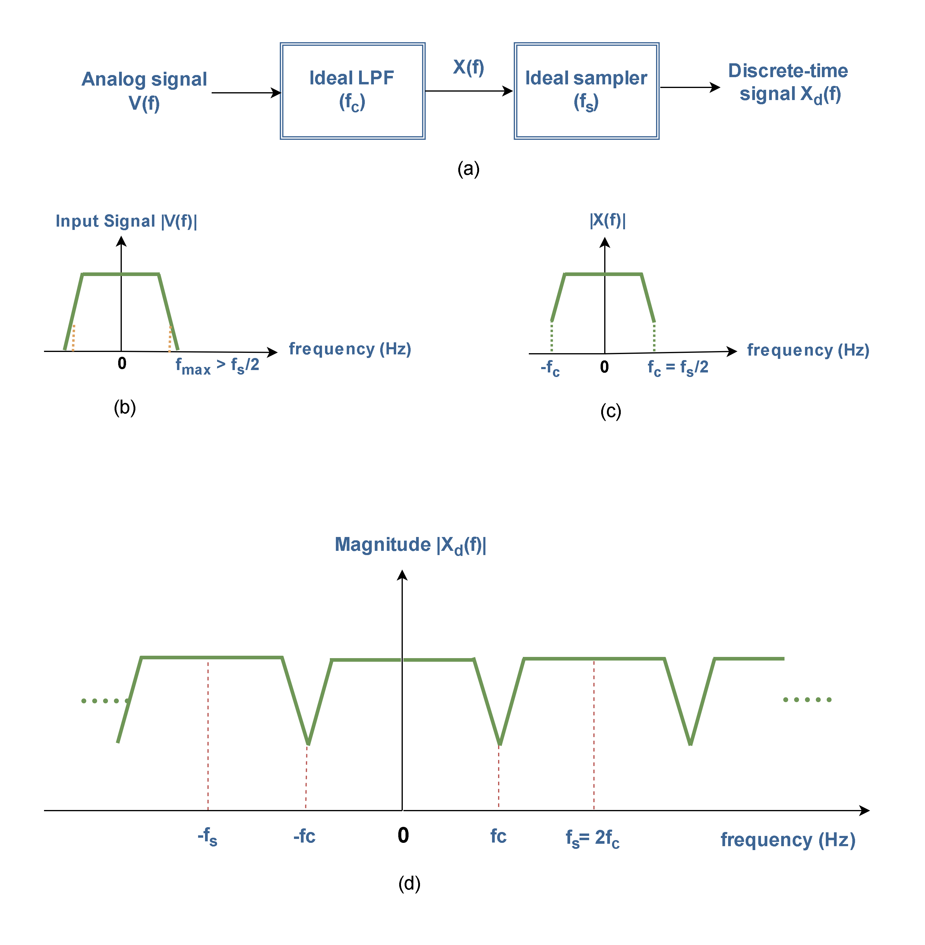
Figure 8: (a) The sampling system including an ideal LPF (b) The spectrum of the input signal (c) The spectrum of the signal after filtering (d) The spectrum of the filtered signal after sampling
As it is depicted in Figure 8 (d), the resulting replicated spectra of the discretely sampled signal [Xd(f)] do not overlap each other. Thus, no aliasing occurs.
Quantization
The quantization stage (Figure 9) rounds off the value of samples to the nearest discrete amplitude values in a set of L quantum levels. This process is lossy (not reversible) since it is not possible to determine again the exact value of the original fractional number from the rounded integer.
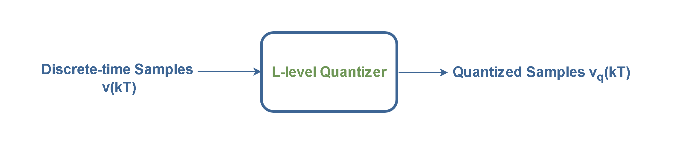
Figure 9: The L-level quantization stage
As well as the sampling process is done along the x-axis (time), and the quantization process is done along the y-axis (amplitude). The spacing between quantization levels is called the quantization width or the quantizer step size which is denoted by q. If the spacing between these levels is the same throughout the range of amplitudes, then it is called a uniform quantizer. A linear quantizer performs a uniform mapping between input and output values.
The following operations are performed in the Quantization stage:
The system assumes that input values, v(t), have amplitudes between Vmin and V Then, for inputs after sampling we have the variable v(kT) as it is explained in Equation 3.
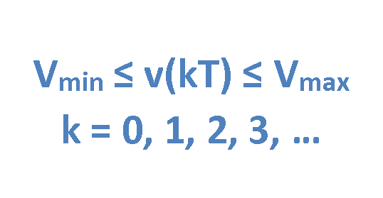
Equation 3: The range of amplitudes
The system divides the range of amplitudes into L quantization levels, each of size q as described in Equation 4.
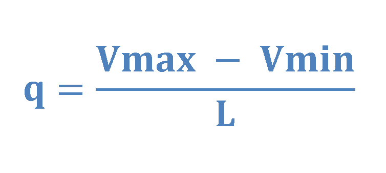
Equation 4: The value of quantization width
The number of quantum levels for a binary PCM system must equal some power of 2, as it explained in Equation 5 (We will see the reason in the next step).
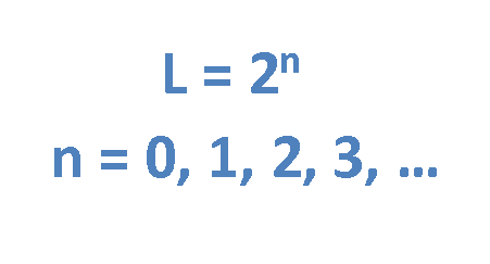
Equation 5: The number of quantum levels
A simple example of quantization is the mechanism of rounding a fractional number to the nearest integer as it is described in Equation 6.
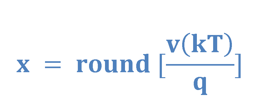
Equation 6: The quantization as rounding a fractional number to the nearest integer
Then, the quantized results come out from Equation 7.
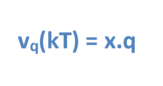
Equation 7: Calculation of quantum levels
Figure 10 shows the characteristic function of the typical uniform quantizer relating to our example waveform in Figure 3.
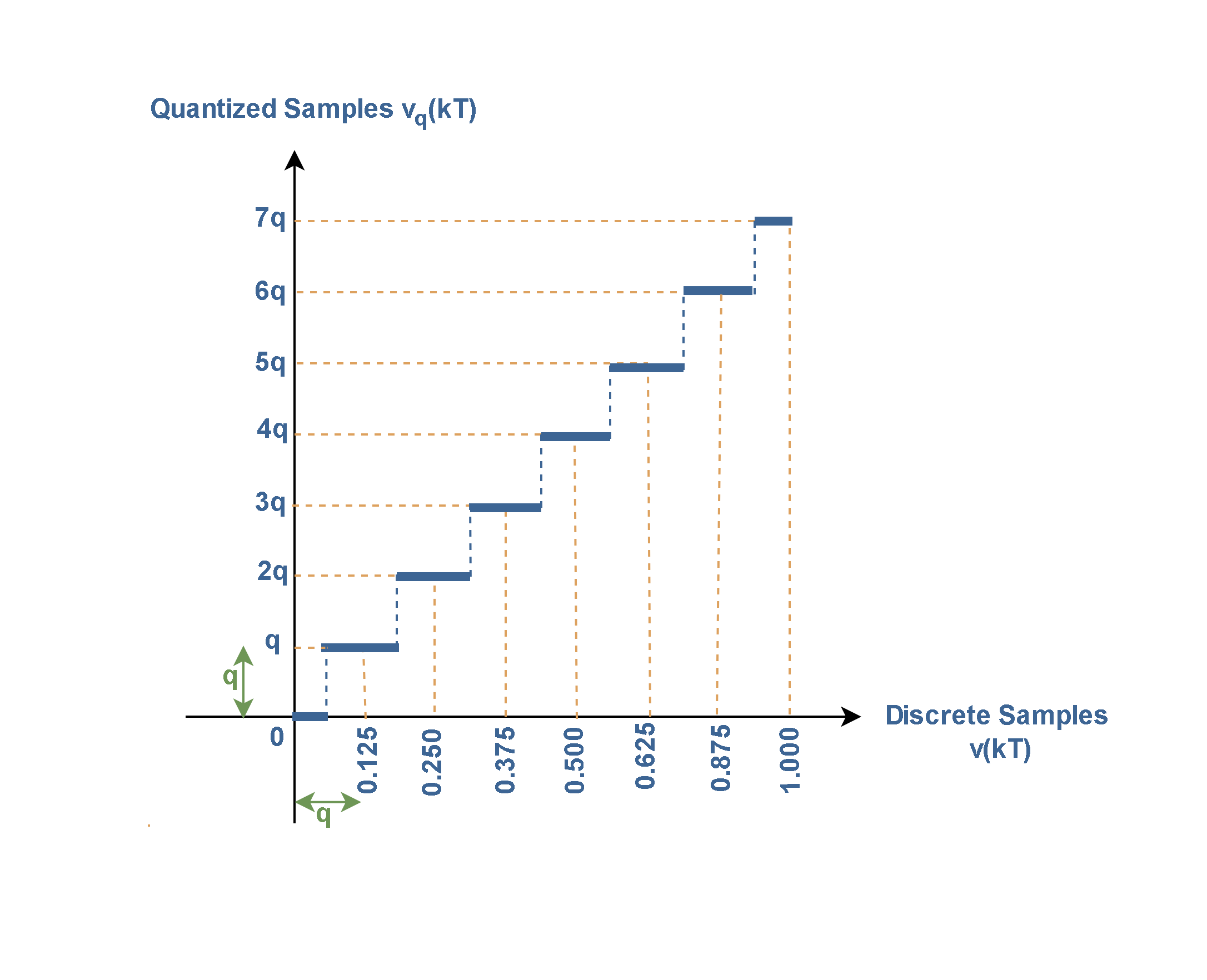
Figure 10: the characteristic function of a uniform quantizer
In this graph, some new levels in equal distances with integer values are defined as quantized levels for output results. In this case, because of 8 levels of quantization between 0 and 1 volts, the quantity q equals to (1/8), equivalent to 0.125 volts of the amplitude.
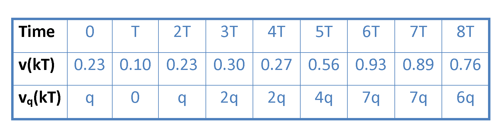
If we apply Equation 6 on the samples of v(kT) in Figure 3, we can collect the calculated data of quantization in Table 1.
Table 1: Quantization data of our example
The output results of Table 1 are plotted in Figure 11.
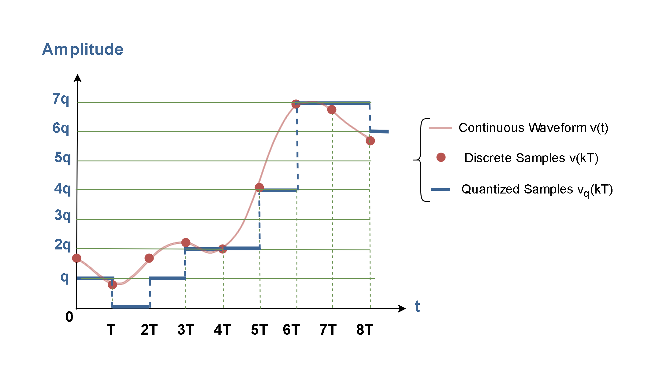
Figure 11: The plot of 3 waveforms (continuous, discrete, and quantized)
Figure 11 shows how the amplitude of the input samples [v(KT)] is mapped to the new quantization levels of amplitude at the output. Also, it is clear that the first continuous waveform v(t) is replaced by the new discrete waveform [vq(kT)].
It is important that the shape of the quantized-samples function vq(kT) (the blue curve) could be a discrete approximation for the original continuous waveform v(t) (the red one), but it also could be better by increasing the number of quantization levels to 16 or 32 and so on.
Summary
- Essentially, analog signals are continuous in both time and amplitude. Analog signals, during the time interval within which they are measured, can have any amplitude (including zero) between the minimum and maximum limits, for every instant of time.
- The amplitudes of discrete-time signals are determined only at certain time instants.
- Digital signals are non-continuous. They are discrete both in time and amplitude. They jump from one allowed value to another as time moves on. There are a limited number of values.
- In practice, computers are best able to work with what is known as digital signals.
- The most common technique to change an analog signal to digital data is called pulse code modulation (PCM). A PCM encoder has the following three processes: Sampling, Quantization, and Encoding
- The result of ideal sampling is a series of sampled values between the maximum and minimum of the input signal.
- The number of measurements (amplitude samples) taken per second is known as the sampling frequency. The terms sample rate and sample frequency are often used interchangeably and are usually denoted by fs.
- According to the Nyquist theorem, the sampling rate must be at least 2 times the highest frequency contained in the signal. It is also known as the minimum sampling rate and is given by: fs =2 fmax
- If the sampling frequency is smaller than twice the highest frequency of the spectrum (fs < 2fmax) a unique form of distortion called alias distortion, is produced.
- Anti-aliasing filters are always analog low-pass filters as they process the signal before it is sampled.
- In the quantization stage, the system replaces each original sampled value with the nearest quantization level.
- In the quantized signal, only a finite number of amplitudes are measured at distinct points in time.
- The number of values, or voltage levels (L), in a digital system, is determined by the number of bits (n) in each binary number: Number of voltage levels = L = 2n
- The quantization step size is denoted by q.


