The Fourier Analysis –The Fast Fourier Transform (FFT) Method

Introduction

The Fourier Transform is a mathematical technique that transforms a time-domain signal into its frequency-domain representation. In other words, it decomposes a signal into its frequency components. The result is called the spectrum of the signal. Historically, the Fourier analysis concept developed slowly, from the Fourier series method 200 years ago up to the Discrete Fourier Transform (DFT) computing method today. Essentially, the Fourier decomposition was unsatisfyingly slow, often requiring several minutes to execute on present-day computers. The Fast Fourier Transform (FFT) is a family of algorithms developed in the 1960s to reduce this computation time.

The discovery of the Fast Fourier Transform (FFT) by J. W. Cooley and John Tukey in 1965, revolutionized signal processing. Cooley and Tukey are credited with introducing the FFT to the world in their paper: “An algorithm for the machine calculation of complex Fourier Series”, Mathematics Computation, Vol. 19, 1965, pp 297-301.

In practice, we often deal with discrete signals, which are represented as a sequence of samples taken at discrete time intervals; digital computers work with such signals. The discrete Fourier transform (DFT) applies to signals that are discrete in time and aperiodic. Based on the Fourier analysis theory, an aperiodic signal is composed of an infinite number of sines and cosines. The DFT is defined as the sum of the product of the signal values and complex sinusoidal functions (called basis functions) at different frequencies.

The direct computation of the DFT involves nested summations or recursive computations, making it computationally expensive. The O() notation is used to describe the worst-case scenario of the algorithm’s time complexity. It provides an asymptotic upper limit on how the running time increases as the input size (number of samples) grows. The time complexity of a direct DFT implementation is O(N²), where N is the number of discrete samples in the signal. This means, that in such a scenario in which the algorithm would involve nested loops, it results in a quadratic growth in running time as the input size (N) increases.

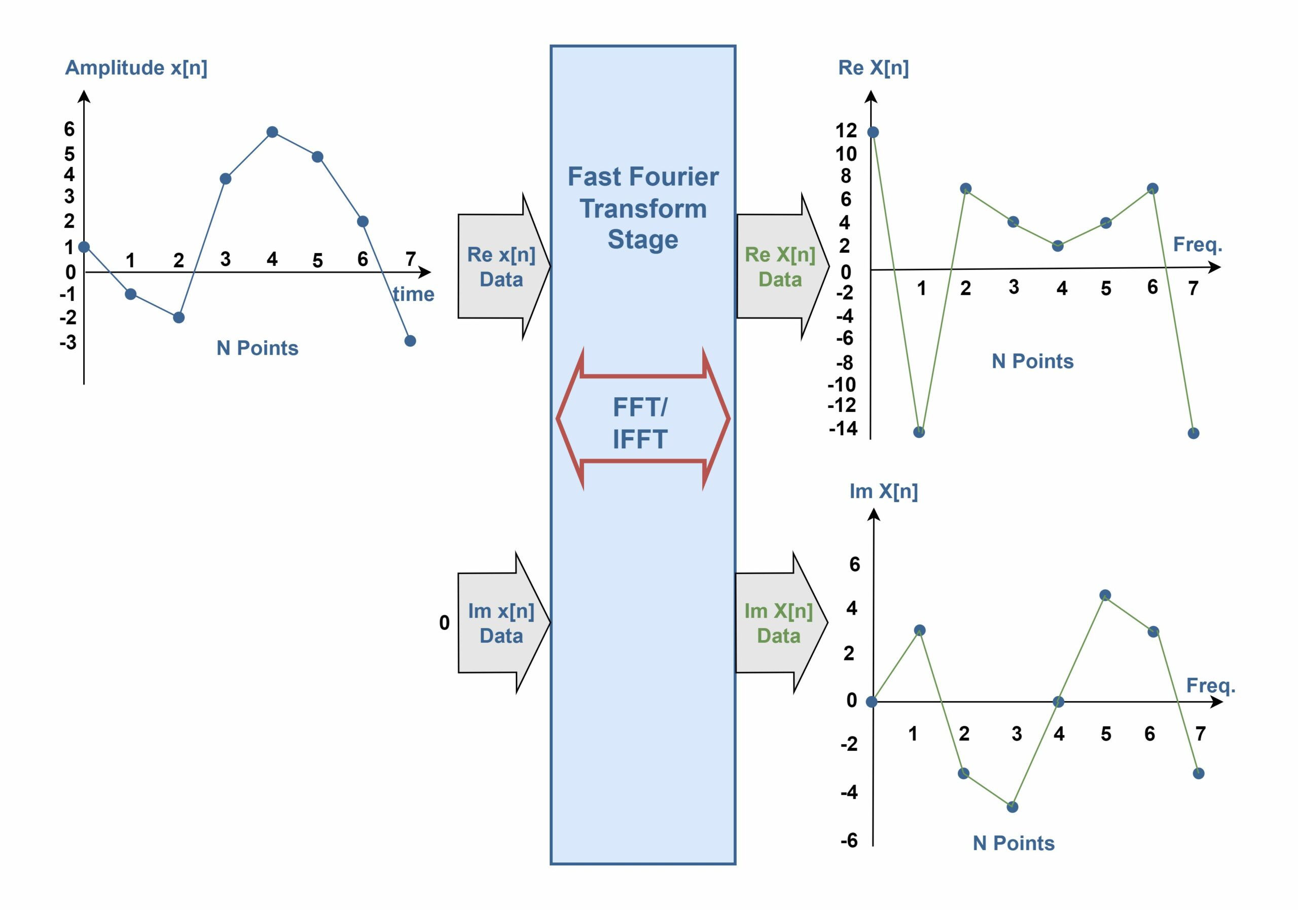
The FFT as an algorithmic technique made the computation of the Fourier transform simpler and quicker and finally allowed Fourier analysis to be recognized and used more widely. In this method, by eliminating duplicate computations in the DFT, it became possible to produce the frequency spectrum of a signal with N data points in (N.log₂N) operations. This made real-time digital signal spectrum analysis feasible. Figure 1 shows a general example of the FFT operation on a small sequence with 8 samples.

The Fast Fourier transform has been widely used in the field of digital signal processing. Back in 1988, a 256-point FFT still consumed minutes of PC time. Today, an 8192-point FFT (8k FFT) takes less than one millisecond of computing time! This opens the door for new and interesting applications such as digital video and audio compression and test engineering or Orthogonal Frequency Division Multiplex (OFDM) in telecommunication systems. In modern storage oscilloscopes, the FFT makes it possible to perform a low-cost spectrum analysis. The FFT has also been used in the field of acoustics and geology.

Review Of Discrete Fourier Transform (DFT)

In the previous article, we considered the DFT method:

The Fourier Analysis – Discrete Fourier Transform (DFT)

The forward complex discrete Fourier transform (DFT) of x, also known as the spectrum of x, is defined by Equation 1.

This is more commonly written as Equation 2.

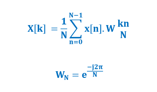
and, W_N for k = 0 … N−1, are called the Nth roots of unity. The sequence X[k] is the discrete Fourier transform of the sequence x[n]. Each is a sequence of N complex numbers which are composed of two numbers, the real part and the imaginary part. For example, the complex sample X[15],  refers to the combination of Re X[15] and Im X[15]. Then, Equation 1 (or 2) saves a lot of additions and multiplications, as complex operations, not real.

However, the DFT can be solved by simple mathematical and numerical means and it functions both forwards and in the reverse direction in the time domain (Inverse Discrete Fourier Transform – IDFT). Similarly, Equation 3 describes the method of inverse calculation.

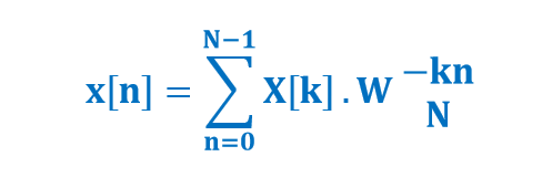
The result of performing a DFT on a real-time domain signal interval is a discrete complex spectrum (real and imaginary parts). The IDFT transforms the complex spectrum back into a real-time domain signal again.

The Fast Fourier Transform (FFT)

The Discrete Fourier Transform is a simple but fairly time-consuming algorithm. However, if the number of points N within the window of observation is restricted to N = 2^m, i.e. a power of two, a more complex but less time-consuming algorithm can be used, which is called the Fast Fourier Transform (FFT). This algorithm provides the same result as a DFT but is much faster and restricted to N = 2^m points (2, 4, 8, 16, 32, 64, 128, 256, 512, 1024, 2048, …).

It is important to clarify that the DFT and FFT are not completely different entities. The FFT is a collection of efficient algorithms for calculating the DFT with a significantly reduced number of computations. The Discrete Fourier Transform and the Fast Fourier Transform are all defined through the field of complex numbers. The Fast Fourier Transform can also be inverted (Inverse Fast Fourier Transform – IFFT). Figure 2 describes the FFT numerical structure.

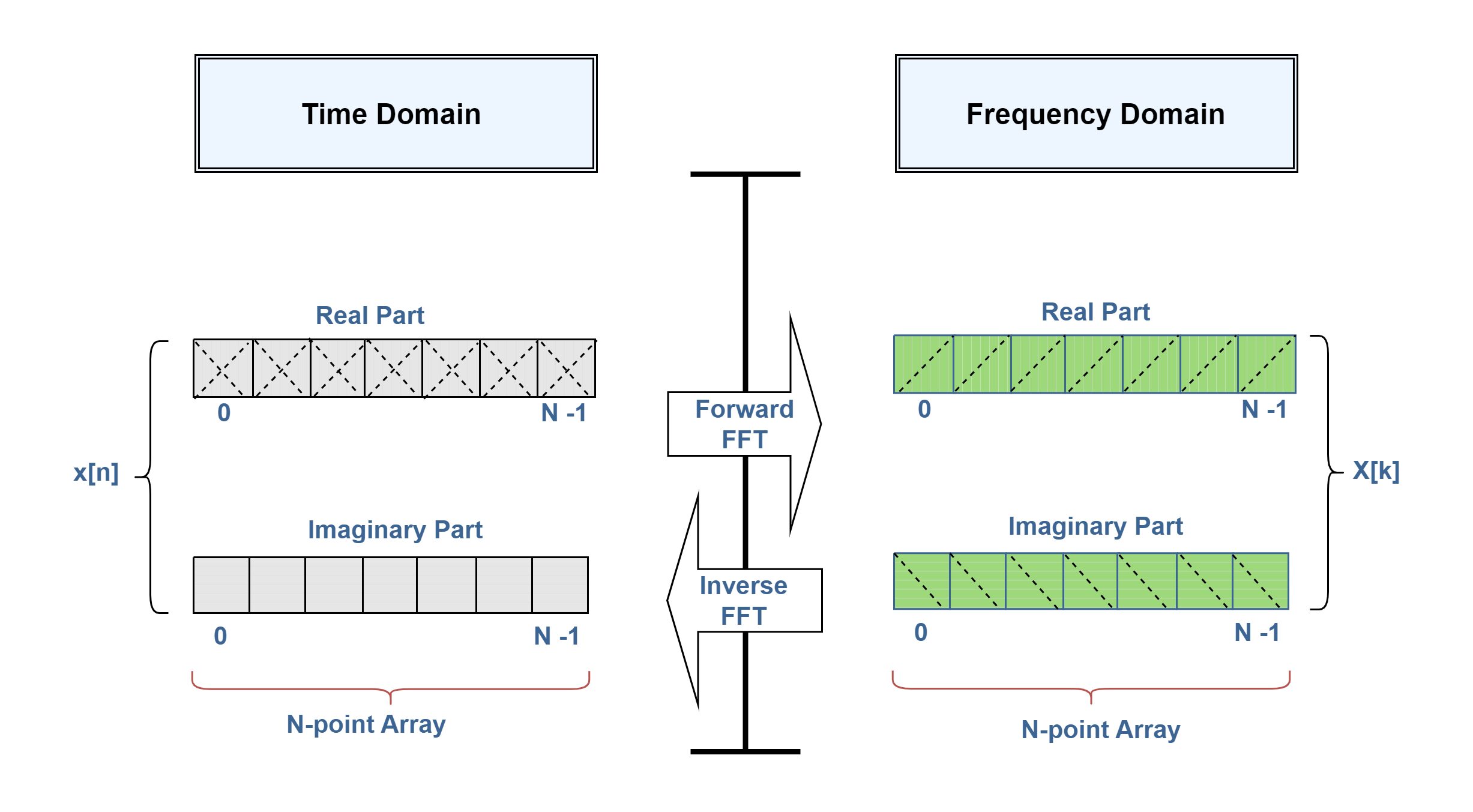
The complex FFT transforms two N point time domain signals into two N point frequency domain signals. The two time-domain signals are called the real part and the imaginary part, just as are the frequency-domain signals. Despite their names, all of the values in these arrays are just ordinary numbers. (The j’s are not included in the array values! They are a part of the mathematics of complex numbers).

As the N samples of a typical time domain signal are always purely real, the corresponding imaginary part must be set to zero for each of the N points. This means that the imaginary-part table for the time domain must be filled with zeros.

Mechanism Of The FFT Operation

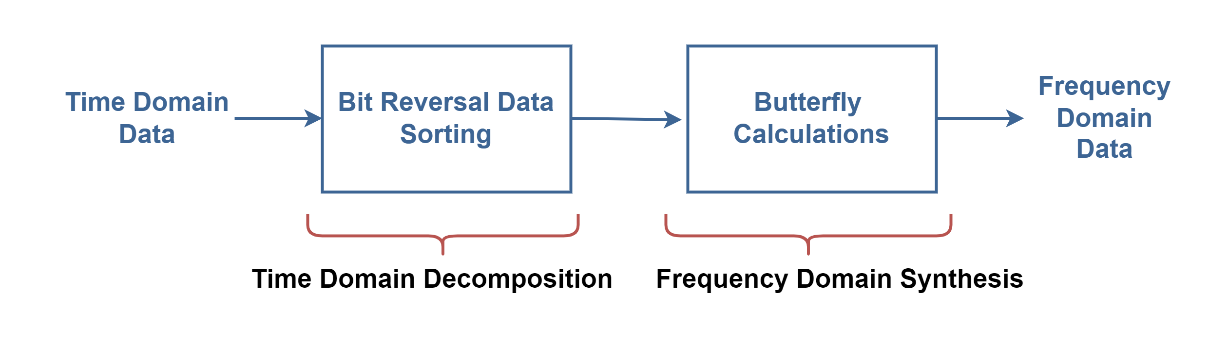
The FFT is an algorithmic approach to compute the DFT which exploits the symmetry and periodicity properties of sinusoidal functions to speed up the computations. The FFT makes use of methods of linear algebra. The samples are pre-sorted in co-called bit reversal and then processed using butterfly operations. These operations are implemented as machine codes in signal processors and/or special FFT chips.

Let’s review the method of the Fast Fourier Transform:

• The FFT algorithm efficiently exploits the fact that for a power-of-2 size signal (N = 2^m), the DFT can be expressed in terms of smaller DFTs.
• The fundamental principle behind the FFT algorithms is to divide the computation of the DFT of N samples into successively smaller DFTs, recursively compute their solutions, and then combine these solutions to get the final DFT result.
• The Cooley-Tukey algorithm is one of the most widely used FFT algorithms and the Radix-2 decimation-in-time (DIT) is the simplest and most common form of the Cooley–Tukey algorithm.
• Decimation involves dividing the input sequence into smaller sub-sequences, which are then processed recursively to compute the FFT.
• Radix-2 DIT divides a DFT of size N into two interleaved DFTs (hence the name “radix-2”) of size N/2 with each recursive stage.
• The algorithm operates by decomposing an N point time domain signal into N time domain signals each composed of a single point. The second step is to calculate the N frequency spectra corresponding to these N time domain signals.
• The Radix-2 FFT has a time complexity of O(N.log₂N), which is a significant improvement over the O(N²) complexity of the direct DFT.

The first step of the Radix-2 decimation-in-time (DIT) procedure is the time domain decomposition of input samples. Figure 3 shows an example of decomposition used in the FFT for the case of N = 8. On the left, the indexes of the original signal samples are listed along with their binary equivalents. On the right, the rearranged sample numbers are listed similarly.

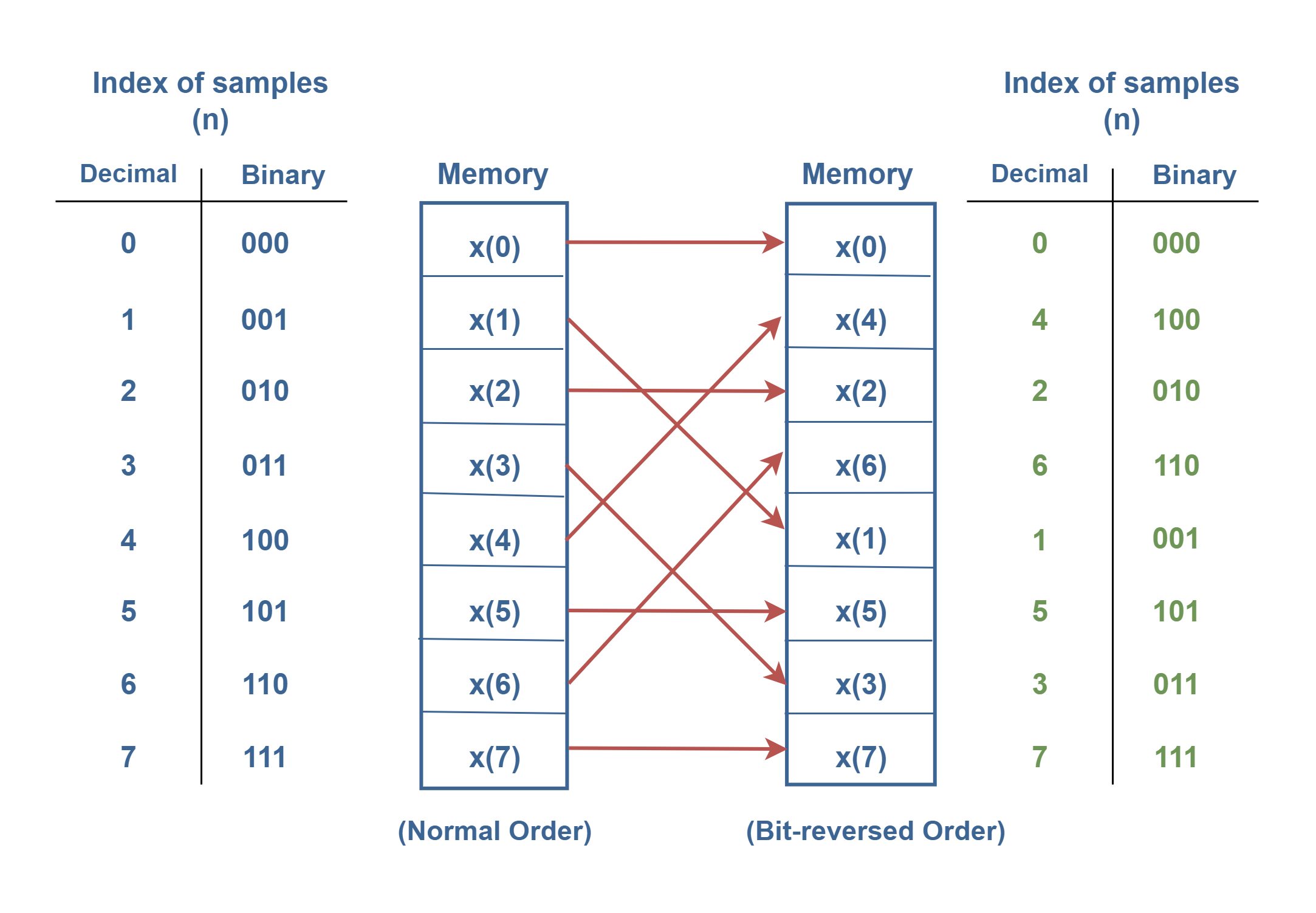
An interlaced decomposition is used each time a signal is broken in two, that is, the signal is separated into its even and odd sample indexes. Essentially, the decomposition is nothing more than a reordering of the samples in the signal.

The important idea is that the binary numbers are the reversals of each other. For example, sample number 3 (011₂) is exchanged with sample number 6 (110₂), and so forth. Some of the sample numbers also remained unchanged, like 0 and 7. Then, the FFT time domain decomposition is usually carried out by a bit reversal sorting algorithm. This involves rearranging the order of the N time domain samples by counting in binary with the bits flipped left for right. The data x[n] after decomposition is stored in bit-reversed order. Figure 3 shows the required rearrangement pattern.

Figure 4 shows the FFT butterfly. This is the basic calculation element in the FFT, taking two complex points and converting them into two other complex points by addition and multiplication operations. This simple flow diagram is called a butterfly due to its schematic shape.

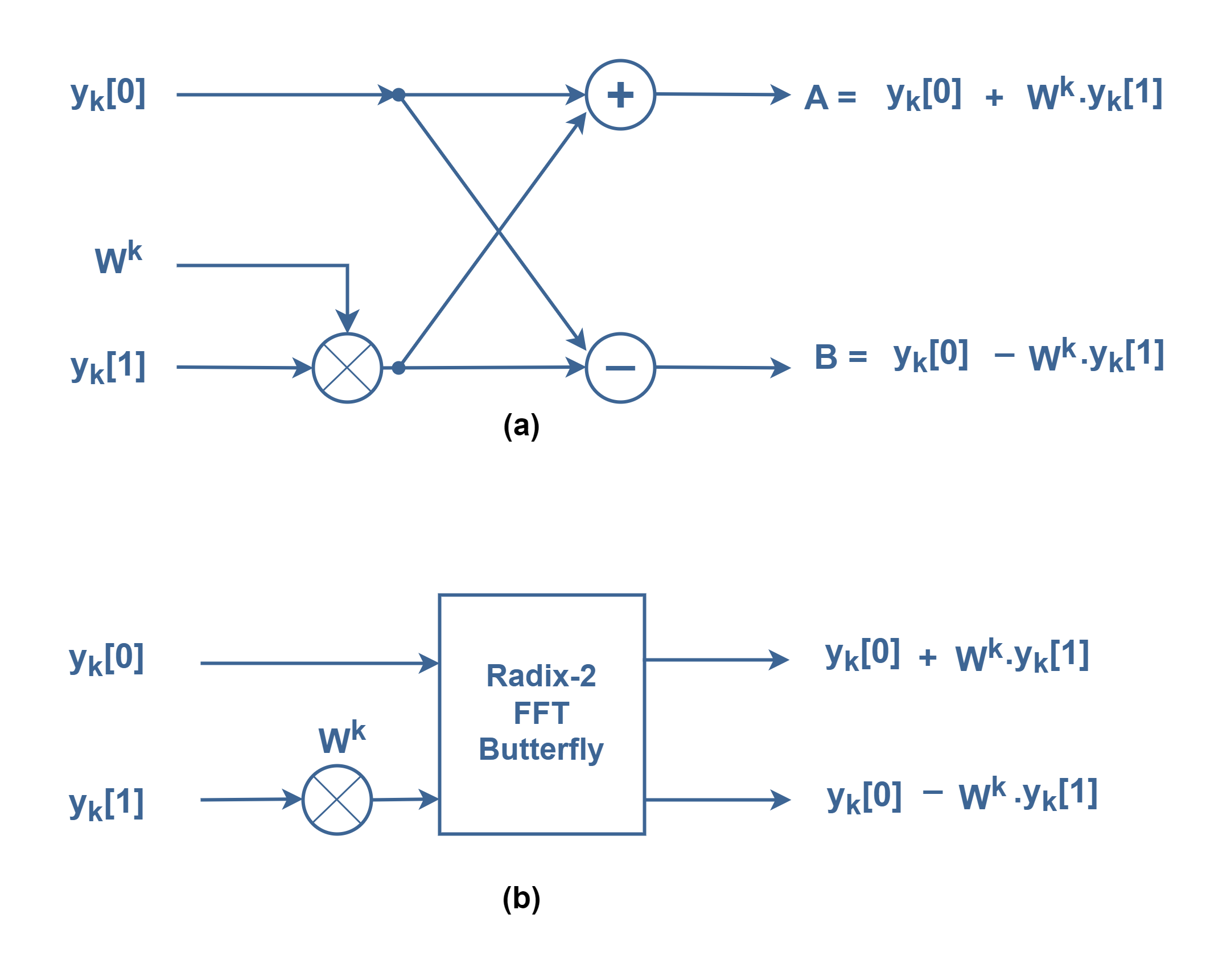
This typical FFT butterfly operation involves two complex numbers as inputs, denoted as y_k[0] and y_k[1]. The operation transforms these two values into two new values, (y_k[0] + W^k. y_k[1])  and (y_k[0] – W^k. y_k[1]), following specific mathematical rules. We can call the results, for example, A and B. Then, the butterfly operation computes new values for sum and difference as described in Equation 4.

In Equation 4, W is a complex root of unity. In the Cooley-Tukey Radix-2 FFT, W is a twiddle factor that depends on the size of the FFT and the stage of computation.

The butterfly operation is then repeated recursively in different stages of the FFT algorithm, ultimately leading to the efficient computation of the DFT. Understanding the butterfly operation is crucial for grasping the inner workings of the FFT algorithm, and it provides insight into how the FFT efficiently decomposes and combines frequency components during its computation.

Figure 5 shows the general idea behind the FFT algorithm and how to produce the N-point frequency spectra from the N-point time domain data.

Let’s go through an example of computing a 4-point FFT (N= 4) using the Cooley-Tukey Radix-2 FFT algorithm. For N= 4, the twiddle factor W is W₄ = e^−2πi/4 =​ e^-πi/2.

Step-By-Step Calculation For N=4 FFT

Start The Algorithm

We start with the original input sequence with arbitrary values {x[0], x[1], x[2], x[3]} and we define samples with even and odd indexes.

Stage 1:

The FFT butterfly operations at this stage involve twiddle factor W₄ raised to the power of 0.

Butterfly 1

• In the first butterfly operation, we combine x[0] and x[2] as samples with even indexes.
• x[0] and x[2] are added and subtracted, respectively, using the twiddle factor W⁰.

Butterfly 2

• In the second butterfly operation, we combine x[1] and x[3] as samples with odd indexes.
• x[1] and x[3] are added and subtracted, respectively, using the twiddle factor W⁰.

Stage 2:

Now, we perform the butterfly operations again using twiddle factor W₄ raised to the power of 0 or 1.

Butterfly 1

• We run another set of butterfly operations, combining the outputs from the previous stage.
• The result of (x[0] + x[2]) is combined with (x[1] + x[3]), using the twiddle factor W⁰.

Butterfly 2

• (x[0] – x[2]) are combined with (x[1] – x[3]) using W¹.

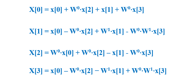
The Final Result

The final sequence X which contains {X[0], X[1], X[2], X[3]}, is the Fourier Transform of the original sequence x. The method of computation is explained by Equation 5. The results are equal to the DFT results.

Visualization Of Butterfly Mechanism

Let’s visualize the butterfly mechanism for the FFT computation with N=4. In this case, we have two stages of computation. Each stage involves two butterfly operations. The procedure is plotted in Figure 6. The arrows represent the flow of data through the butterfly operations. Each butterfly operation combines two inputs and produces two outputs.

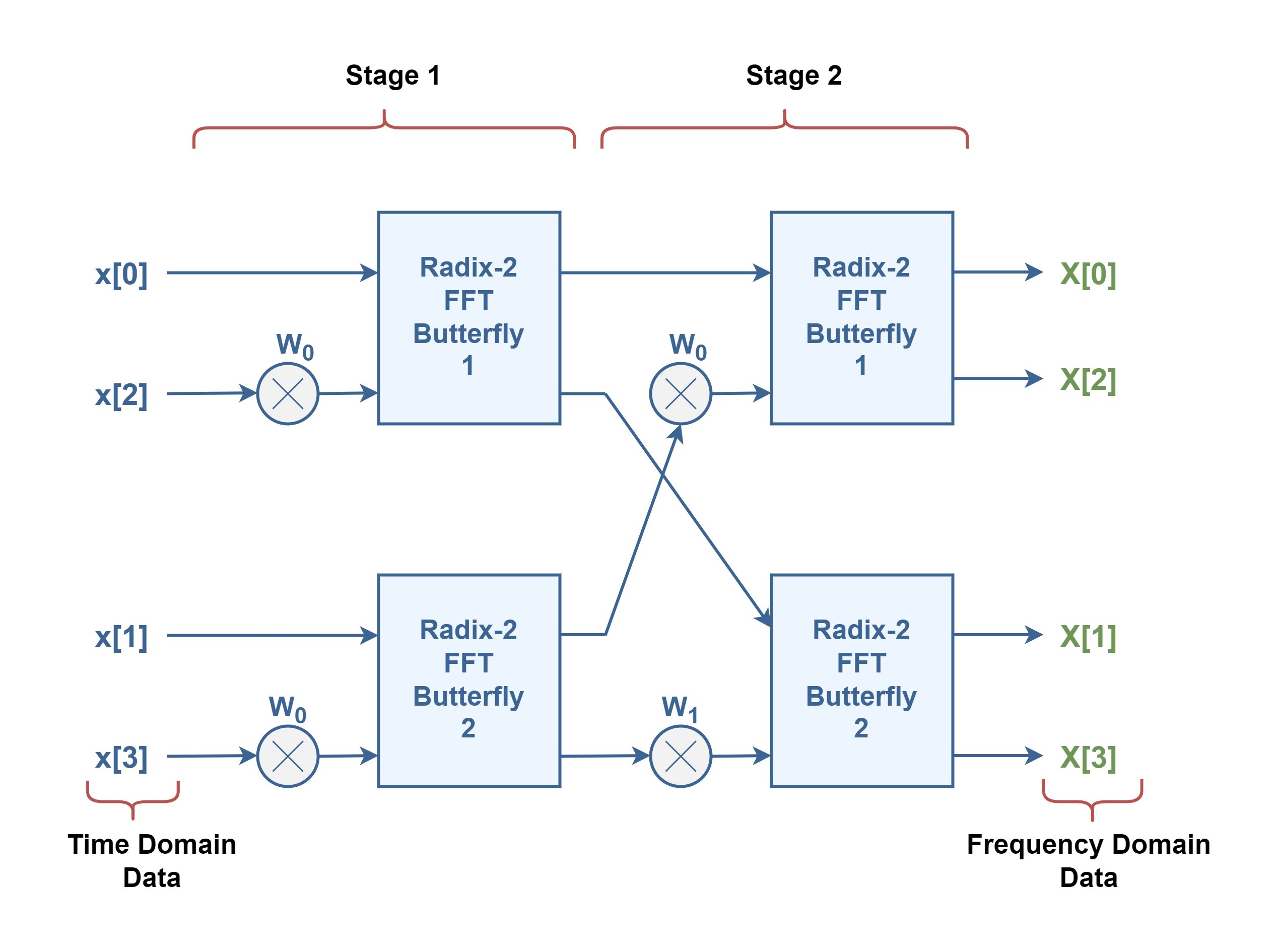
In the FFT computation process, the number of outputs is always equal to the number of inputs, and it matches the size of the input sequence. Therefore, for N=4, we have four input elements (x[0], x[1], x[2], x[3]) and four corresponding output elements (X[0], X[1], X[2], X[3]).

Example Calculation

We can consider a realistic example by calculating the FFT for the input sequence x = {1, 2, 3, 4}. Based on the above-mentioned Equation and using (W⁰ = 1) and (W¹ = -j), we can find the solution as explained in Table 1.

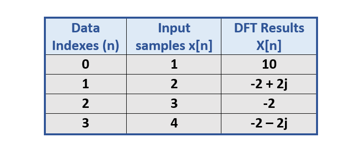
This simple example illustrates the basic steps of the FFT algorithm for N= 4. In practice, for signals with many more elements (N >> 4), the FFT algorithm efficiently performs the transformation of these operations using a recursive strategy, reducing the overall computational complexity.

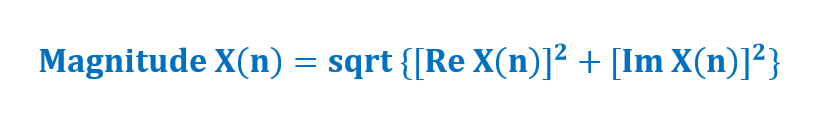
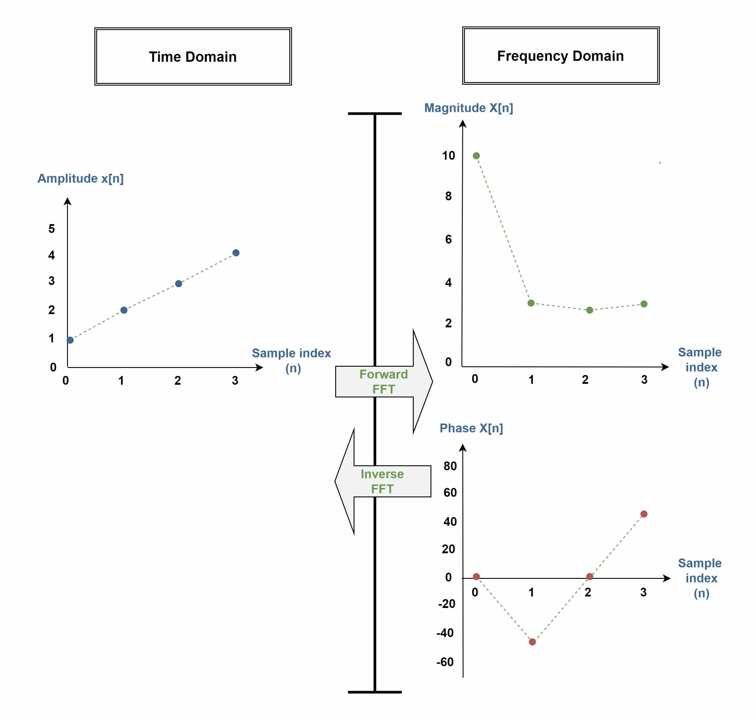
Spectrum Of The Signal Based On FFT Calculations

To generate a frequency domain plot from this data, the magnitude and the phase of each complex sample must be calculated using Equations 6 and 7.

The results of the calculation are summarized in Table 2.

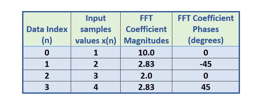
The results are then plotted in Figure 7. In the graph, the horizontal axis is the frequency in terms of sample indexes, and the vertical axis is the amplitude. A 0 frequency component indicates the amplitude of the DC component of a signal which is the sum of all the sample values in the sequence.

Comparison Of Computational Complexities Between DFT And FFT Methods

If N samples are given to a DFT, the time it takes to compute the amplitudes of the sinusoids is proportional to N². But, the Radix-2 FFT algorithm requires only N·log₂N complex operations. For example, for a 1024-point transform, the DFT requires 1,048,576 complex operations compared to only 10,240 for the FFT.

Table 3 shows the speed improvement of the FFT over that of the DFT in terms of different values of N.

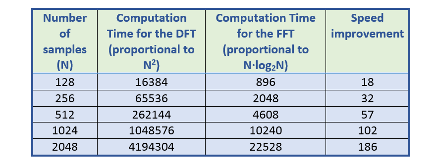
It is clear that the speed improvement is quite significant for larger values of N and this is the main efficiency of the FFT for real discrete signals with large sizes, like N = 1024 and so on.

Summary

• The Fast Fourier Transform is an efficient algorithm for computing the discrete Fourier transform (DCT), and its speed is crucial in applications like signal processing, audio analysis, image processing, and many more where the frequency domain information of a signal is needed.
• The FFT (Cooley, Tukey, 1965), an algorithmic technique, made the computation of the Fourier transform simpler and quicker and finally allowed Fourier analysis to be recognized and used more widely.
• The key idea is to break down the computation into smaller DFTs recursively, taking advantage of the symmetry and periodicity properties.
• The butterfly operation is a fundamental operation and a key element employed by FFT to efficiently compute the discrete Fourier transform (DFT).
• A butterfly operation combines two points in the frequency domain, performing a specific computation involving addition and multiplication. The butterfly operation is called so because, when depicted graphically, the data flow diagram resembles the shape of a butterfly.
• The most common version of FFT is the Radix-2 FFT, where the size of the input signal is a power of 2 (N = 2^m).
• The Cooley-Tukey Radix-2 FFT algorithm, one of the most commonly used FFT algorithms, employs the decimation-in-time (DIT) approach.
• Typical time domain signals are, however, always real, i.e. the imaginary part is zero at every point in time. The imaginary part must be set to zero before the Fourier transform or its numerical variations FFT are performed.
• The recursive application of these operations reduces the overall computational complexity of the FFT algorithms.
• Compared to the direct DFT computation complexity of O(N²), the FFT, utilizing the Cooley-Tukey algorithm, achieves superior time complexity of O(N.log2 N), rendering it more suitable for larger input sizes due to its reduced computational demands.

Please follow and like us: