Harmonics

Introduction

Periodic signals are not always perfect sinusoidal patterns such as presented in one of our previous tutorials about Sinusoidal Waveforms. Sometimes, signals can indeed be a superposition of simple sine waves and they are known as complex waveforms.

In this tutorial, we will focus on complex periodic waveforms to understand what they consist of and how they can be analyzed.

First of all, we present the concept of harmonics along with the spectrum representation. In the second section, we focus on spectral analysis, which is the mathematical tool to analyze harmonics, based on the Fourier series.

Presentation

Consider a periodic signal s(t) which is a superposition of two sinusoidal waveforms called harmonics y₀(t) and y₁(t) which their frequencies and amplitudes satisfy ω₁=2ω₀; A₀=2A₁. Their expressions are therefore given by y₀(t)=A₀sin(ω₀t) and y₁(t)=A₁sin(ω₁t). Figure 1 illustrates the harmonics y₀(t) and y₁(t) separately from the resulting signal s(t) :

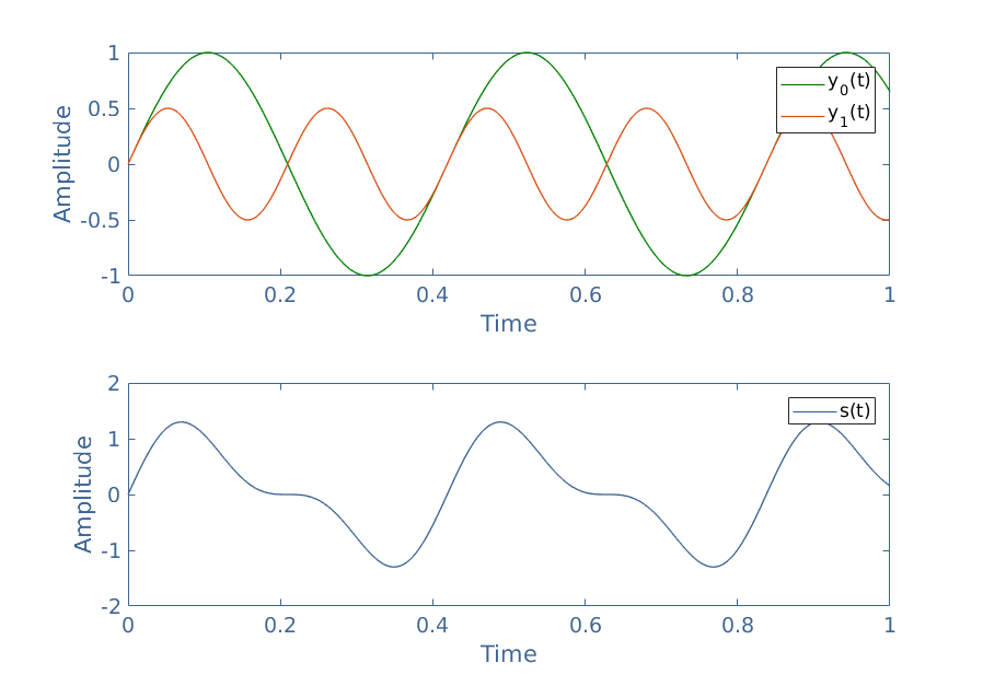
In this example, y₀(t) is called the fundamental harmonic and y₁(t) the first harmonic. The fundamental harmonic is the signal with the lower frequency and it gives the periodicity of the resulting signal s(t): we can indeed see that ω₀=ω_S.

Harmonics are therefore the “building” functions of a complex waveform, however, their frequencies are not random and always satisfy ω₀=ω_S, ω₁=2ω₀, and ω₂=3ω₀ if a second harmonic is present and so on … In the general case, the frequency of the n^th harmonic satisfy the relation ω_n=(n+1)×ω₀.

When given a particular complex waveform, one representation is very suitable and called the spectrum of the signal. This representation consists of plotting the amplitudes of each harmonic as a function of the frequency and can be computed by a numerical program such as Python or MatLab :

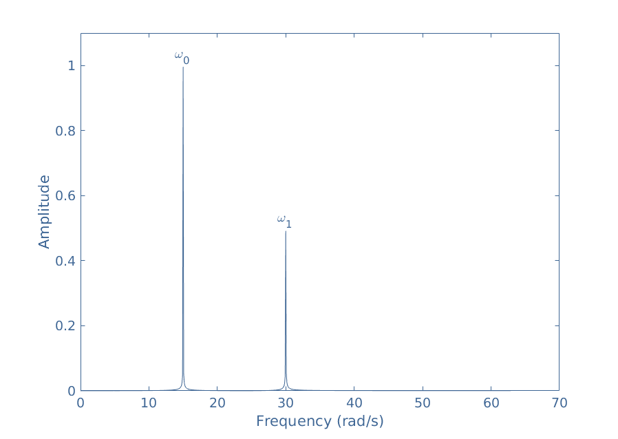
Examining the spectrum of s(t), it is clear to visualize that the fundamental signal has a frequency f₀=15/2π=2.4 Hz and an amplitude A₀=1 (V or A for example) while the first harmonic has a frequency of 2f₀=4.8 Hz and an amplitude A₁=0.5.

Spectral analysis

Plotting a spectrum such as shown in Figure 2 is based on a mathematical tool known as the Fourier’s series. It is in the early 19th-century that this method is developed by the French scientist Joseph Fourier and it is still nowadays one of the major tools of signal analysis.

This method is based on the observation that any periodic signal y(t) is, in fact, an infinite sum (a series) of harmonics which amplitudes and phases can be computed. The same observation can be written as a mathematical equation :

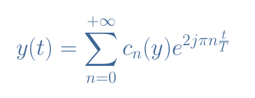
The complex exponential term is simply the complex form to write the harmonics (refer to the tutorial Complex Numbers). The integer n refers to the n^th harmonic and T is the periodicity of y(t).

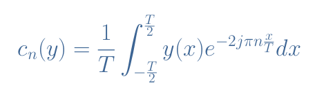
The coefficients c_n(y) are called Fourier coefficients of the function y(t) and are determined by the following relation :

It is common to split the coefficients c_n into two coefficients a_n and b_n, which for real functions are given by :

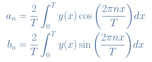
This method to determine the Fourier decomposition of any periodic signal, therefore giving the spectrum such as presented in Figure 2 is also known as Fourier Transform (FT) which is an extension of the same method for non-periodic signals.

Two cases need to be considered separately in order to proceed to an FT of a periodic signal and explained in the following subsections.

Known signal

The first case is if the signal to be decomposed has a known analytical expression. Consider for example a square signal sq(t) with a periodicity of T. Its expression is known through the following definition :

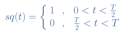
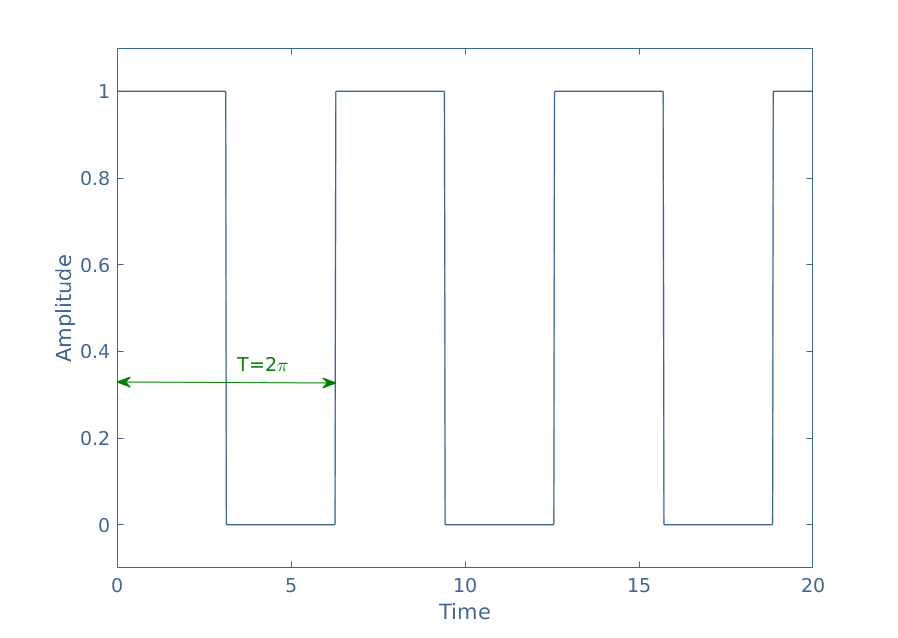
Figure 3 represents a square signal of period T=2π over a few periods :

First of all, we determine the expression of the term a₀ :

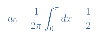
This coefficient represents the average value of the signal: y(t) and is indeed equal to 1 for half of the time and 0 otherwise. Note that since sin(0)=0, the term b₀ is equal to zero.

When developing the expression of a_n for n>0, we realize that these coefficients are proportional to sin(nx) evaluated between 0 and π, which is alway equal to 0, therefore (a_n)_n>0=0.

Finally, we determine the general expression for the coefficients b_n for n>0:

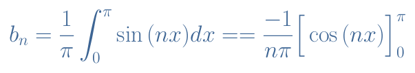
When evaluated between 0 and π, the term cos(nx) is equal to -2 if n is odd and 0 if n is even. The final expression of (b_n)_n>0 is therefore given by:

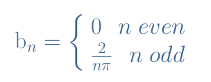
Each coefficient b_n corresponds to the amplitude of the harmonic sin(nt). From the expressions of a₀ and b_n, we can, therefore, give the full Fourier development of the square signal sq(t):

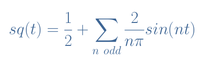
From Equation 4 we can plot a part of the spectrum of sq(t) shown in the following Figure 4:

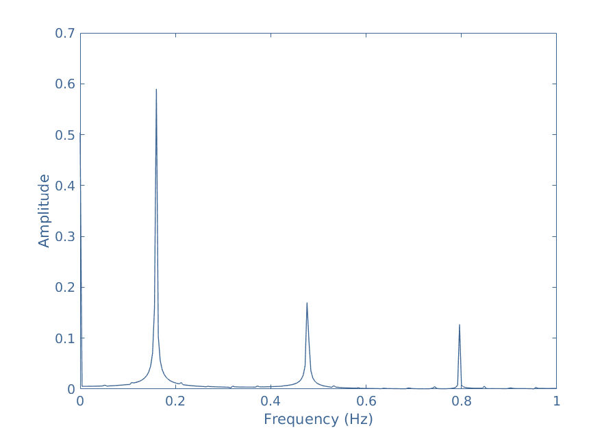
For this signal, only the odd harmonics are present, their amplitude is given by 2/nπ and frequency by n/2π. Note that the average value is also present in the spectrum for a frequency of 0 Hz. Since a square signal presents an infinite number of harmonics, the spectrum is of course shown only until a certain frequency.

When generating a square signal with a function generator for example, only a finite number of harmonics is taken in order to build the waveform. We say that the signal is generated using harmonics until the fifth-order if we use the harmonics 1, 2, 3, 4 and 5 for example, the order gives the degree of accuracy regarding the shape:

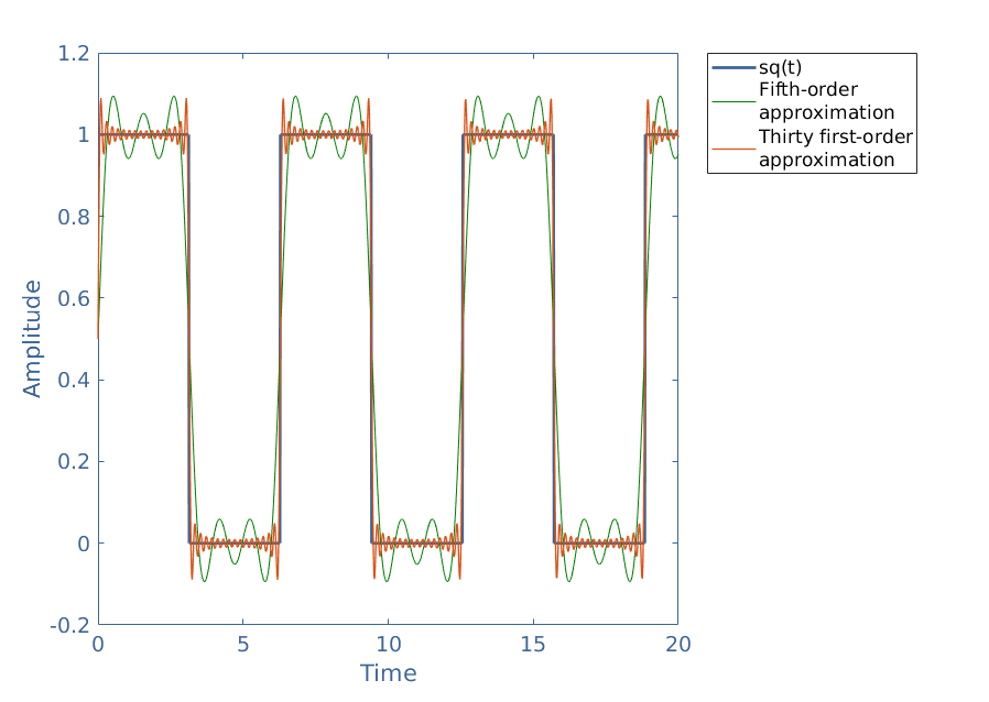
When the order of the approximation increases, we can pinpoint that an overshoot appears around the discontinuity jump (where the signal brutally alternates from 0 to 1 or from 1 to 0). This is known as the Gibbs phenomenon and appears for every signal where a discontinuity jump is present.

Unknown signal

Let’s reconsider the example given in the presentation section and give an explanation of how the numerical program determines the Fourier decomposition of s(t). In Figure 1 we can measure the periodicity of s(t) to be T=0.42 s.

The first coefficient c₀(y) is easy to determine and equal in our example to 0 because the integral over a period of a periodic signal that is symmetrical around the horizontal axis is always equal to 0. Indeed, this first coefficient is always related to a DC quantity and therefore an average value, which is not present in our case.

When the expression of the function s(t) is known, the coefficients c_n can be analytically computed such as shown in the previous subsection. However, for an unknown function s(t), the coefficients a_n(y) and b_n(y) for n>0 are determined by numerically by computing the area between -T/2 and T/2 (or 0 and T) under the curve of the functions s(t)cos(2πnt/T) and s(t)sin(2πnt/T).

This can be done by many methods, one of the easiest to implement and understand is the rectangle method which idea is represented in Figure 6 for the function s(t)sin(2πt/T):

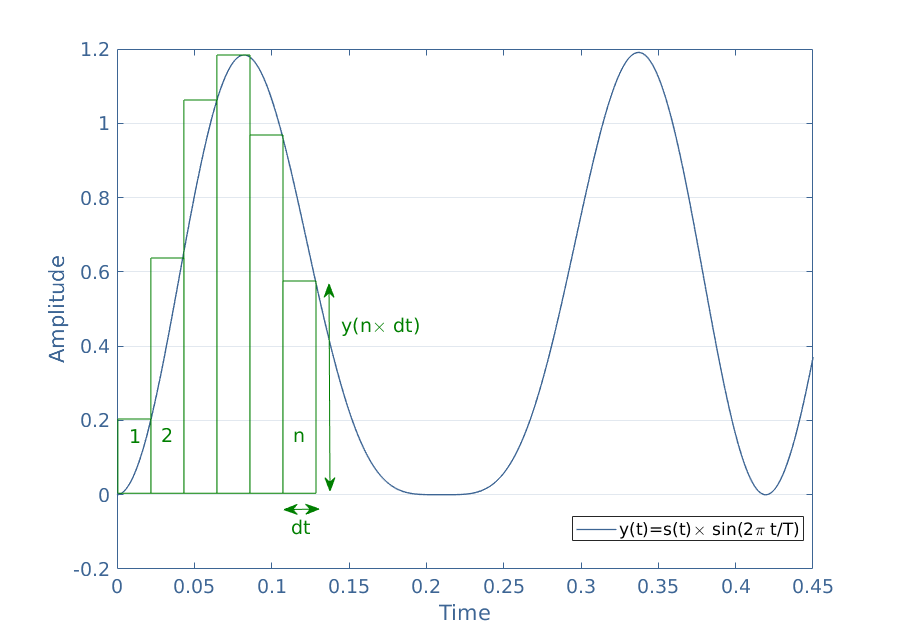
As shown in Figure 5, this method consists of approximating the integral of the curve by summing the area of small rectangles of width dt and height y(n×dt) with n being the index of the rectangle considered.

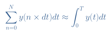
The period T of the signal y(t) is subdivided in N rectangles such as N×dt=T. When dt is small enough, the sum of the area of the rectangles is approximately equal to the integral of y(t) over a period:

It is worth to mention that more precise methods exist in order to converge better to an exact result, such as for example by choosing another shape than rectangles to follow the curve more accurately.

Conclusion

As presented in the first section of this tutorial, harmonics are elementary sine waveforms that form any periodic signal. Some complex waveforms can have a finite number of harmonics and others have an infinite number, such as the square signal presented later in the tutorial.

The frequencies of harmonics are always an integer multiple of the fundamental frequency of the complex signal. Their amplitude usually decreases towards high frequencies and can be determined by the Fourier decomposition.

The spectrum representation is the most convenient way to highlight the harmonics of a signal, it is computed thanks to the Fourier decomposition presented in the second section. The decomposition can be analytical if an expression of the complex waveform is known or numerical if the signal is unknown.

Please follow and like us: