Complex Numbers and Phasors

Introduction

Complex numbers are an important mathematical tool that is widely used in many physics domains, including electronics. The concept might seem odd, but their manipulation is simple and their efficiency notable.

In the first section, general concepts about the complex numbers are presented in order to get familiar with their representation. A second section will follow by enumerating some of the most important definitions associated with complex numbers. After defining some key concepts, the third section will deal more in details with their calculation rules. Finally, we will understand why they are used in electronics and simplify calculations as an efficient tool.

Presentation

This section presents from a pure mathematical point of view the complex numbers and the set associated to. The set of complex numbers is noted ℂ and it is an extension of the usual set of real numbers that we are familiar with. Real numbers are therefore included in complex numbers.

The starting point to define complex numbers is the imaginary unit i also noted j in electronics to avoid confusion with the current. This number is defined such as j²=-1, in some countries or institutions, the notation j=√-1 can also be encountered.

While real numbers can be represented in a 1D space along a line, complex numbers are represented in a 2D space called the complex plane. This structure is represented in Figure 1 below :

Let’s first talk about the complex plane, it consists in two axis where any complex number can be represented. The horizontal axis is the real number set and the vertical axis is the imaginary axis.

As shown in Figure 1, a complex number z can be described by either two real numbers a and b that represent coordinates, or by a distance |z| and an angle θ. The first option to describe z is called the algebraic form and is defined in Equation 1:

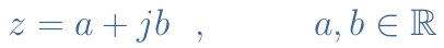
It is interesting to highlight some particular cases. If b=0, z=a, which means that the complex number is reduced to a real number. If a=0, z=jb, in that case, z is called a pure imaginary number.

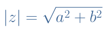
The second way to define z is called the polar or exponential form. Before giving the expression of this form, we need to understand what consists |z| and θ. The value |z|, also called module is the distance between the origin of the complex plane and the complex number. It is defined by the Pythagorean theorem such as shown in Equation 2 :

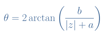
The value θ is called the argument and defines the angle between the real axis and the complex number. Unless a=0 and b=0 or a<0 and b=0, the argument can always be calculated with the following formula :

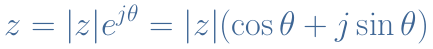
Using Euler’s formula, the polar description of a complex number z is given by a distance and an angle and satisfies the following formula :

Definitions

Many definitions are associated with complex numbers.

Two simple operators are often used in complex algebra: Re and Im. Let’s suppose a complex number z=a+jb, the real part operator Re is defined such as Re(z)=a and the imaginary part operator is defined such as Im(z)=b. Another easier way to determine the argument θ of a complex number with the condition that Re(z)>0 is given by : θ=arctan(Im(z)/Re(z)).

The complex conjugate is another important definition and widely used in complex algebra. The complex conjugate of a complex number z is noted z* and as the same real part but an opposite imaginary part : if z=a+jb, z*=a-jb. In exponential form, if z=|z|e^jθ, z*=|z|e^-jθ. Many relations can be established with the complex conjugates but the most important one is to note that z×z*=|z|².

In the complex plane, the conjugation operation translates to a symmetry with respect to the real axis :

It is interesting to note that if Im(z)=0, z=z* : the complex conjugate of a real number is the number itself. Moreover, the conjugation operation is reversible : (z*)*=z.

Calculation rules

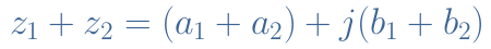
The addition (or subtraction) of two complex numbers z₁=a₁+jb₁ and z₂=a₂+jb₂ consists in separately consider the real and imaginary parts :

Such as for real numbers, the multiplication of complex numbers is distributive and illustrated in Equation 6 after regrouping the real and imaginary parts :

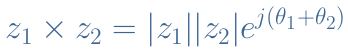
If z₁ and z₂ are written in exponential form, the multiplication operation is even easier to realize :

The division operation with complex numbers is however more complicated to perform, using the algebraic form than with real numbers. Let’s consider the two complex numbers z₁ and z₂ previously defined. The trick to perform a division is to transform the complex denominator into a real denominator. For this, we multiply both the numerator and denominator by the denominator complex conjugate such as shown below :

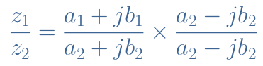
By realizing the multiplication such as shown previously, we get now a complex numerator that can be divided by a real denominator :

Let’s consider the example of z₁=2+4j and z₂=3+j and proceed to the division z₁/z₂ :

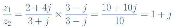
This result, can also be written in exponential form  z₁/z₂=√2e^jπ/4.

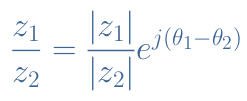
Such as we highlighted for the multiplication operation, the division can be done more easily with the exponential form :

Equation 9 can be verified with the same example. First, we need to calculate the modules and arguments of z₁ and z₂ :

• |z₁|=√2²+4²=√20 and θ₁=Arg(z₁)=arctan(4/2)=arctan(2)
• |z₂|=√3²+1²=√10 and θ₂=Arg(z₂)=arctan(1/3)

The division of the modules gives |z₁|/|z₂|=√2 and the argument of the division is arctan(2)-arctan(1/3)=π/4. The result of the division is therefore √2e^jπ/4 and confirms the result we previously calculated using the algebraic form.

Complex numbers in electronics

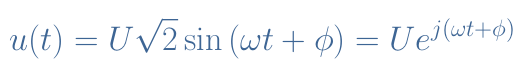
Any periodical signal such as the current or voltage can be written using the complex numbers that simplifies the notation and the associated calculations :

The complex notation is also used to describe the impedances of capacitor and inductor along with their phase shift. It can indeed be shown that :

• Z_C=1/Cω and Φ_C=-π/2
• Z_L=Lω and Φ_L=+π/2

Since e^±jπ/2=±j, the complex impedances Z^* can take into consideration both the phase shift and the resistance of the capacitor and inductor :

• Z_C^*=-j/Cω
• Z_L^*=jLω

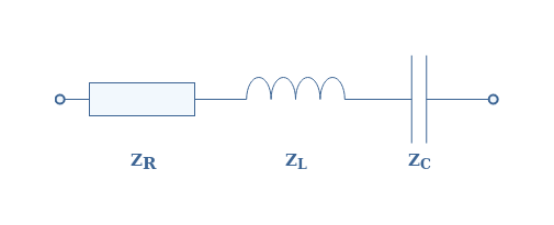
We can consider as an example a simple RLC circuit in serie with its associated complex impedances Z_R, Z_L and Z_C. The total complex impedance is therefore : Z_RLC=Z_R+Z_L+Z_C=R+j(Lω-1/Cω).

The imaginary part of this impedance is called the reactance and noted X, in this example, X_RLC=Lω-1/Cω. We can distinguish three cases to describe the behavior of a circuit :

1. X=0 means that the circuit is purely resistive : it acts as a resistance and follows Ohm’s law
2. X<0 the circuit is capacitive : it acts as a capacitance and tends to make an opposition to any change of voltage.
3. X>0 the circuit is inductive : it acts as a inductance and provokes an opposition to any change of current.

The total impedance of the RLC circuit is given by the module of Z_RLC which is : |Z_RLC|=√(R²+X_RLC²).

The phase shift between the voltage and current is given by the argument of Z_RLC which is : Arg(Z_RLC)=arctan(X_RLC/R).

Both the impedance and phase shift depend on the frequency of the signals. This evolution can be represented using MatLab® in Figure 3 where the components have been chosen such as R=1 kΩ, L=10 mH, C=20 μF.

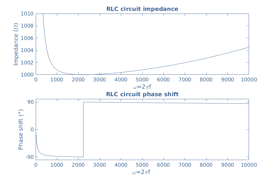
We can note that first the circuit is capacitive since it presents a negative phase shift and becomes inductive after a certain frequency value. This remark can be validated by plotting the reactance in Figure 4 where it is shown that the shift between negative and positive values occurs for the same particular frequency :

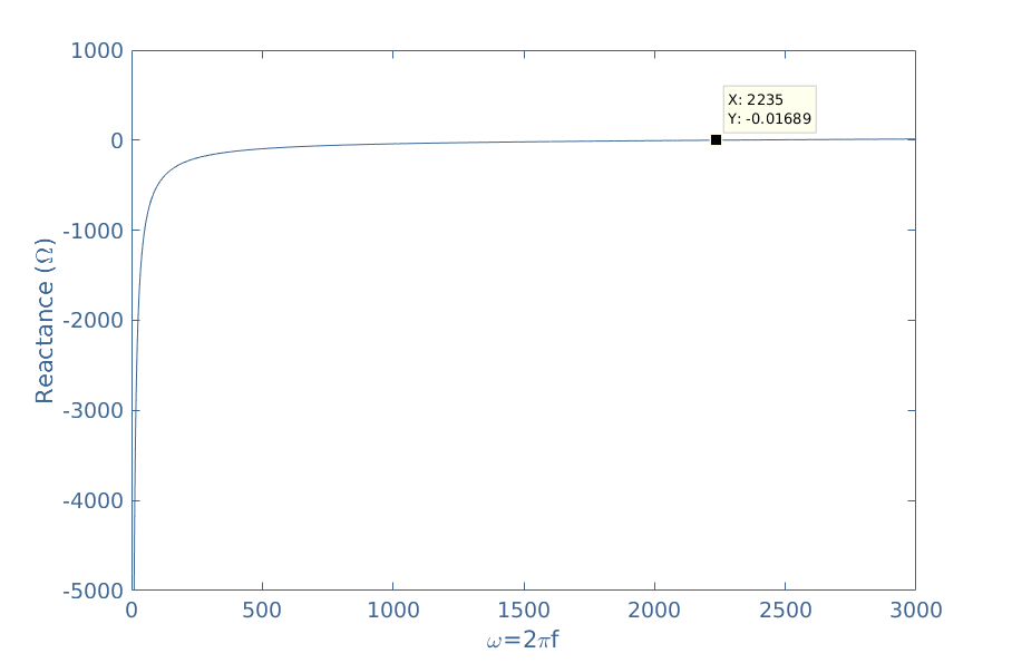
This particular frequency f₀=2235/2π=356 Hz is called the resonance frequency of the circuit and satisfies X=0. In our example, X_RLC=0 ⇒ ω₀=1/√LC=2235, which is confirmed by the value highlighted in Figure 4.

Conclusion

Complex numbers have emerged since nearly 500 years and have been built by some of the most brilliant mathematicians such as Gauss or Cauchy. Since then, they are used in many scientific domains such as electronics and it’s a powerful tool.

In the very first section, the concept of complex numbers is presented. The complex set can be seen as a plane where each number can be defined by coordinates (algebraic form) or a distance and angle (exponential form). Complex numbers have the property to be solutions of some equations that cannot be solved by usual real numbers, such as the equation x²=-1. Some more important notions such as the conjugation transformation are introduced in a second section.

The calculation rules are presented in a third section. We have seen that the addition, subtraction and multiplication are very similar with real and complex numbers. However, the division operation requires more steps, involving the use of the conjugation transformation.

Finally, we have seen how complex numbers can be used in electronics to describe periodical signals, impedances and determine the behavior of circuits in frequency-dependent regimes.

Please follow and like us: