Average and RMS voltage

Introduction

In the DC regime, only one definition of the value of a voltage is possible, this value is unambiguous and is determined by the difference between the reference value 0 V and the flat line figure of the DC signal.

In the AC regime, however, it can lead to confusion to speak of only one value for the voltage. From a simple sine waveform, we can at least list indeed four different definitions of voltage:

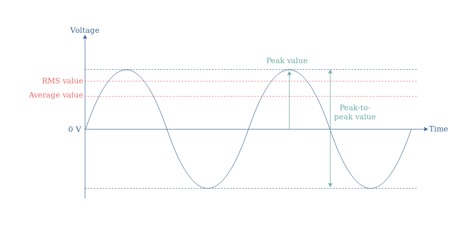
The peak value corresponds to the difference between the reference (which is the value where the AC signal oscillates around) and the maximum value of the signal. The peak-to-peak value is the peak value multiplied by a factor 2, it corresponds to the total vertical width of the signal.

In Figure 1, we have also highlighted the Average and RMS values in red, which we will be focusing on in the following of this tutorial.

The two sections developed in this article will separately present the Average and RMS values, we will see how they are defined, how to determine them and finally we will see what is special about the RMS value.

Average Voltage

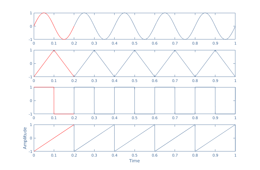
For an elementary symmetrical sine, triangle, square or sawtooth waveform (see Figure 2 and AC Waveform tutorial), it is unclear to speak of the average voltage value, that we will note A in the following. Indeed, these types of signals are during half of their period positive and negative during the other half. In other words, the signals are 50 % of the time above the horizontal axis and 50 % under it.

From that observation, it is easy to understand that if we consider the average value of any of these signals on a full period, it is equal to 0, regardless of the peak value, and therefore not relevant.

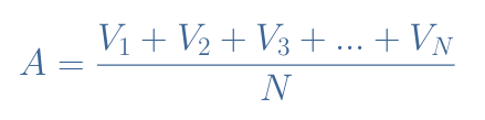
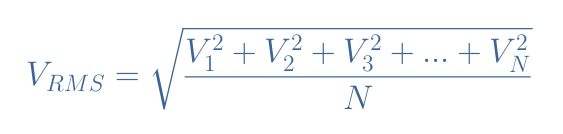
We can demonstrate this result by explaining how to calculate the average value. For a finite set of values, the averaging process consists of summing all the values (V₁, V₂, V₃…)  and dividing them by the cardinal number N of the set (how many values there are in the set):

For an analog signal, however, it is impossible to sum all the instant values, also called mid-ordinates, that the signal takes during a period simply because there is an infinity. Instead of summing, we use the integration operation:

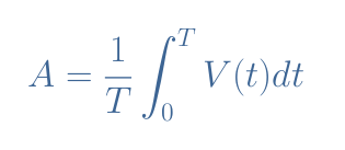
Equation 1 is the average of the signal V(t) taken between the times 0 and T, that is to say, a full period. The term ∫V(t)dt gives the value of the area between the curve V(t) and the reference of 0 V. Because the integration operation is linear, this term can be split in two:

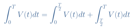
For an elementary waveform such as presented in Figure 1, we can see that the first and second terms of this formula are equals but of opposite signs, therefore the average value is equal to 0.

In order for the average value of such signals to make sense, we prefer to consider separately the half positive and negative periods, which some their values are respectively highlighted in red and green in the following Figure 3:

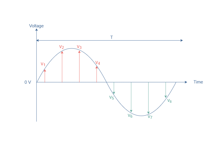
Similarly to Equation 1, we can define separately the average values for the positive half-period (A₊) and negative half-period (A_–):

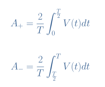
The value of A₊ and A_– depends on the signal we are dealing with and their respective peak values (V_p)_. We list below the absolute value |A| of A+ and A_– for the most common elementary and symmetrical AC signals:

• Sine waveform: |A|=0.637×V_p
• Triangle waveform: |A|=0
• Square waveform: |A|=V_p
• Sawtooth waveform: |A|=0.5×V_p

We can conclude this section by saying that when we want to average a signal, we need to give the precision if the process is done on a full period or a smaller value. For the elementary and symmetrical AC signals, averaging on a full period always gives the result 0 V regardless of the frequency, peak value or period. For this reason, it is more appropriate to average these signals during their half-periods.

RMS Voltage

RMS stands for Root Mean Square, is it a similar operation to the average value presented previously but the instant values are instead squared and the total fraction is rooted:

For the same reasons as stated previously, we use the integration operation to define V_RMS for an analog signal:

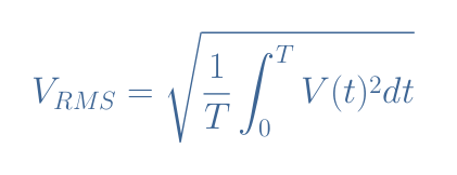
Unlike the average value, the RMS value is always defined for a full period of the signal, there is indeed is no possible confusion to determine this value.

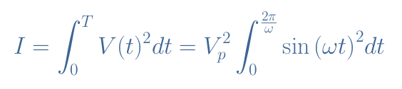
As an example, let’s determine the RMS value of a sine waveform of peak value V_p and angular pulsation ω V(t)=V_p×sin(ωt). We note f the frequency that satisfies f=ω/2π and T=1/f the period.

First of all, we compute the integral term that we note I:

We use the trigonometric identity sin²(x)=(1-cos(2x))/2 to continue:

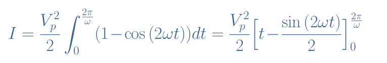
Evaluating the bracket term between 0 and T gives 2π/ω=T. Therefore, the integration term is finally equal to (πV_p²)/ω. From Equation 4 we can see that we still need to multiply by 1/T which leads to [(πV_p²)/ω]×[ω/(2π)]=V_p²/2 for the term under the root.

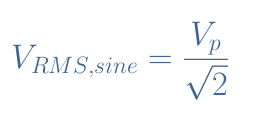
Finally, after taking the root, the final expression for the RMS value of a sine waveform is given by:

We list below the RMS values that can be computed by the same method as the sine example above for the elementary and symmetrical signals stated in the previous section:

• Sine waveform: V_RMS=V_p/√2
• Triangle and Sawtooth waveform: V_RMS=V_p/√3
• Square waveform: V_RMS=V_P

It is important to note that V_RMS>|A|, the RMS value is always greater than the absolute value of the average.

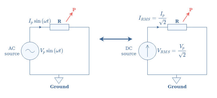
What is fundamental to understand the RMS value is that it creates a link between the DC and AC regimes according to the following Figure 4:

Conclusion

The average and RMS values can easily be measured by modern voltmeters or oscilloscopes and provide information about an AC signal.

The numerical approach for the average consists of summing all the values of a signal and divide the sum by the number of values. For real signals, we prefer to use the integration operation which is an extension of the sum for an infinite set of values.

Two definitions are possible for the average value, depending on if the average is done on a full period or a half-period. Symmetrical signals are characterized by an average value of 0 on a full cycle. The average value on a full cycle is different from 0 only if a DC component is present in the signal or if the signal is not symmetrical around a horizontal reference. Averaging on a half-period can also be done in order to characterize differently symmetrical signals.

The RMS value is defined similarly to the average value but each value of the sum is instead squared and the final result is rooted. The root-mean-square value is always higher than the absolute value of the average and established a link between the AC and DC regimes, which is why it is particularly used by engineers.

Please follow and like us: