Series RLC Circuit Analysis

Introductio

The resistor (R), inductor (L), and capacitor (C) are the three elementary passive components of electronics. Their properties and behavior have already been detailed in the AC Resistance, AC Inductance, and AC Capacitance tutorials.

In this article, we will focus on the series association of these three components known as the series RLC circuit. First of all, a summary of the AC behavior of the three constitutive components is given in a presentation section along with a short introduction to the RLC circuit.

In the second section, we discuss the electrical behavior of this circuit submitted to a DC voltage step and highlight why this particular response is important.

Next, we focus on the AC response of the RLC circuit by computing and plotting its transfer function in a third section.

Finally, we present two alternatives to the RLC circuit by switching the component between each other, and we see that the AC response gets completely different.

Presentation

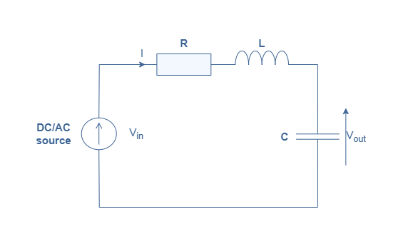
A representation of the RLC circuit is given in Figure 1 below:

The resistor is a purely resistive component that presents no phase-shift between the voltage and current across it. Its impedance (Z_R) remains the same in DC and AC regime and is equal to R (in Ω).

The inductor is a purely reactive component with a phase-shift of +90° or +π/2 rad. Its impedance is given by Z_L=jωL with ω being the angular pulsation of the voltage/current in an AC situation and L is the inductance (in H). In the DC regime, an inductor behaves as a short-circuit between two terminals and in the AC regime it becomes an open-circuit as the impedance increases with the frequency.

The capacitor is also a purely reactive component, but its phase-shift is -90° or -π/2 rad. Its impedance is given by Z_C=-j/Cω with C being the capacitance (in F), it behaves therefore as an open-circuit in DC regime and as a short-circuit in AC regime when the frequency increases.

In Figure 1, these three components are interconnected in series. The circuit is either supplied with a DC or AC source and the output is the voltage across the capacitor. The total impedance of the circuit is the sum of the independent impedances previously stated:

Z_RLC=Z_R+Z_L+Z_C=R+j(Lω-(1/Cω))

In the next section, we present the response of this circuit to a voltage step also known as the transient response.

Transient response

In this section, we will focus on the behavior of the circuit presented in Figure 1 when applying a Heaviside step H(t) to it:

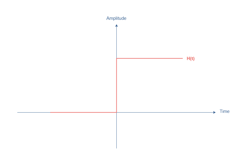
The Heaviside step is characterized by being equal to 0 for t<0 and V_in for t>0. The transition between these two states is similar to an impulsion since the derivative tends to +∞ when t=0.

By doing a mesh analysis on the circuit, we can write that V_in=R×I+L×dI/dt+V_out. Moreover, we know that the current can be rewritten I=C×dV_out/dt, which leads to the following second-order differential equation:

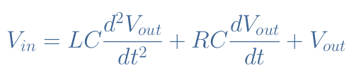
The solution to such an equation is the sum of a permanent response (constant in time) and a transient response V_out,tr (variable in time). The permanent response is easy and obvious to find, the solution V_out=V_in is indeed a permanent solution of Equation 1.

The transient response is complex to determine and involves many steps that will not be detailed in this article. We will admit that its expression can take three different forms and depends on the value of Q=(1/R)√(L/C) called the quality factor of the circuit. Another important parameter is ω₀=1/√(LC) which is the fundamental pulsation of the circuit.

When Q>1/2, the regime is said to be pseudo-periodic or to be an underdamped response, the transient response can be written with the form V_out,tr=Ae^-αtcos(ωt+Φ). The constants A, α and Φ can be found by considering the initial conditions of the circuit (if the capacitor is charged or not …). The pulsation ω is called the pseudo-pulsation and depends on the fundamental pulsation ω₀.

When Q<1/2, the regime is said to be aperiodic or to be an overdamped response, the transient response takes the form V_out,tr=e^-αt(A₁e^-ωt +A₂e^ωt).

Finally, the last case when Q=1/2, which corresponds to the critical regime or critically damped response. In this case, V_out,tr=(A+Bt)e^-ω₀t.

What is important to keep in mind is that these different solutions dictate how the voltage V_out behaves and tends to its permanent value V_in when a Heaviside step is applied to it:

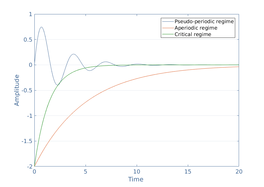
We can comment on this figure by starting to say that each curve tends to 0 when the time increases. It makes sense because we know that V_out=V_in+V_out,tr and V_out(t→+∞)=V_in, therefore, V_out,tr→0.

However, the different possible transient responses do not tend to 0 with the same speed and behavior. The critical regime is the regime that tends the fastest to 0 meanwhile the aperiodic regime is the slowest. The pseudo-periodic regime presents oscillations which amplitude decreases exponentially.

AC response

We consider in this section the same circuit presented in Figure 1 now supplied with an AC source. Using the property that in the complex notation, dX/dt=jωX with ω being the angular pulsation of the source, we can rewrite Equation 1 under the following form:

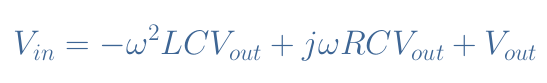
We can then express the ratio V_out/V_in which is the transfer function T of the series RLC circuit:

Knowing that Q=(1/R)√(L/C), ω₀=1/√(LC) and considering the parameter x=ω/ω₀ called the reduced pulsation, we can rearrange Equation 3 to write the canonical form of the transfer function which simplifies and makes the expression more compact:

It is interesting to plot the norm of the transfer function in order to obtain the gain of the circuit as a function of the parameter x. The values R=10 Ω and 20 Ω, L=0.2 H, and C=100 μF have been taken for this example:

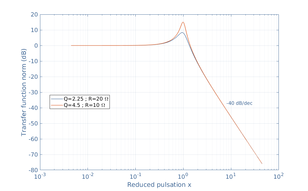
We can note that the series RLC circuit presented in Figure 1 acts as a second-order low-pass filter in the AC regime since it decreases the output signal for the pulsations higher than ω₀, which is commonly called the resonance frequency of the circuit.

It is highlighted in Figure 4 that the value of Q (which depends on R) as an effect on the shape of the curve. The peak around the resonance frequency is indeed characterized by its bandwidth Δω=ω₀/Q.

In this example, ω₀=223 rad/s and Q=4.5 or 2.25, which gives a narrower bandwidth of Δω=50 rad/s for the orange curve and a wider one of 100 rad/s for the blue curve. We can, therefore, note that the quality factor dictates if the resonance is narrow (large Q) or wide (small Q).

Such as mentioned in the previous section, fitting the transfer function of an unknown circuit with the best possible curve enables us to have access to the properties of the circuit and therefore determine the value of its constitutional components.

RCL and CLR configurations

Other associations of the elementary component R, L, and C can provide different types of filters. We have seen previously that an RLC configuration is a second-order low-pass filter, but what if we switch some components between them?

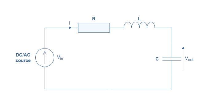
Figures 5 and 6 present two new configurations which will be referred to as RCL and CLR circuits:

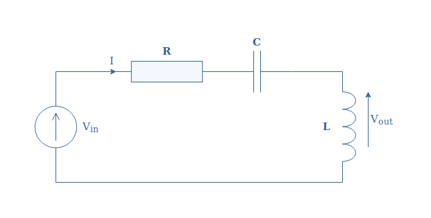
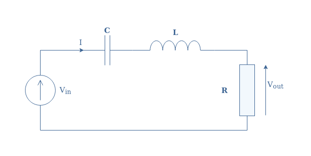
Despite the small changes between these circuits and the original RLC circuit presented in Figure 1, the AC responses are very different.

It can indeed be shown that the transfer functions of these two circuits are given by Equations 4 and 5:

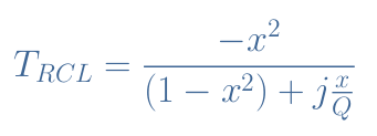
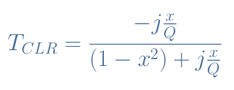
The nature of these new filters is revealed by plotting the norm of their transfer function with the same values: R=10 Ω and 20 Ω, L=0.2 H, and C=100 μF.

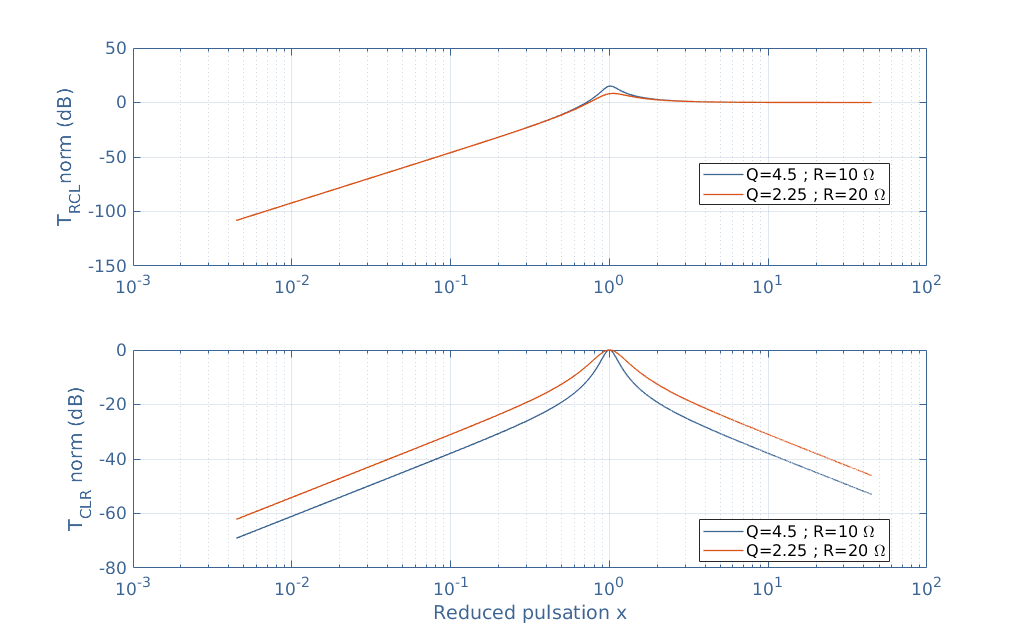
The circuit RCL is a second-order high-pass filter since it attenuates the frequencies under ω₀. The circuit CLR is a band-pass filter since it only amplifies frequencies in around ω₀. Note that the same commentaries as in the previous section about the shape of the curve as a function of Q still apply for both these filters.

Conclusion

The series RLC circuit is simply an association in series of the three elementary components of electronics: resistor, inductor, and capacitor. The impedance of a resistor is a real number and the impedances of the inductor and capacitor are pure imaginary numbers, the total impedance of the circuit is a sum of these three impedances and is, therefore, a complex number.

The transient response of the circuit is first defined and presented in a second section. It consists of investigating the behavior of the circuit when supplied with a Heaviside voltage step. Through studying the possible solutions of the second-order differential equation associated with the circuit, three regimes appear to be possible:

1. The underdamped response where the signal slowly oscillates towards the permanent value V_in.
2. The overdamped response where the signal slowly increases towards the permanent value.
3. The critically damped response is the scenario where the signal increases the fastest towards the permanent value.

In a third section, the AC response of the circuit is presented. When supplied with an AC signal, the differential equation can be written in its complex form in order to find the transfer function of the circuit. Plotting the norm of this function reveals that the series RLC circuit behaves as a second-order low-pass filter.

In the last section, alternative configurations called RCL and CLR are investigated. This section shows that a second-order high-pass filter or a band-pass filter can be made from the same circuit by simply switching the components.

Please follow and like us: