Norton’s Theorem

Introduction

This tutorial is a continuity of our last article about Thevenin’s theorem. In the previous article, we have seen that any linear electrical circuit can be simplified into an elementary circuit that consists of an ideal voltage source in series with resistors.

Another very similar model is known as Norton’s theorem, it has been established in 1926 by the American engineer Edward Norton, more than 70 years after the first version of Thevenin’s theorem.

First of all, we give a recap concerning the bold terms of this sentence in order to understand the appropriate framework where this theorem applies. In the second section, we propose a step by step method to follow in order to determine Norton’s equivalent model of a circuit. Different real examples will be proposed in a third section in order to illustrate this method.

Finally, we will draw a link between Norton’s and Thevenin’s models, before concluding this tutorial.

Presentation and definitions

Linear electrical circuits (LEC) are the framework of Norton’s theorem and they represented a particular type of circuit in which the only components are ideal sources and resistors.

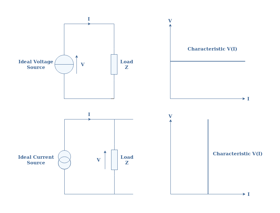
Ideal voltage (resp. current) sources provide a constant value of voltage (resp. current) regardless of the current flowing (resp. voltage) in the circuit. Their representation and behavior are illustrated in Figure 1 below:

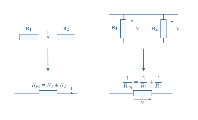
An equivalent resistor R_eq represents an association of a set of interconnected resistors. The rules to associate resistors together are illustrated in Figure 2 below:

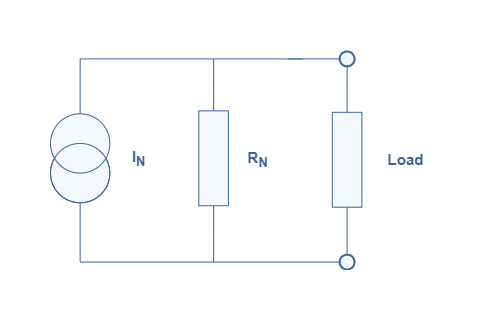
The framework and definition being now clear, we illustrate Norton’s theorem with the following Figure 3:

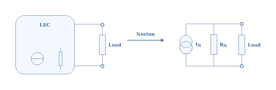
Using Norton’s theorem on a LEC leads to a simple circuit known as Norton’s model composed of an ideal current source in parallel with resistors. The equivalent current source and resistor are labeled with the subscript N as a reference to the name of the theorem.

The next section abstractly presents the step-by-step method to follow in order to determine the Norton model of any LEC.

Norton model determination

Norton’s current I_N represents the current at the terminals of the LEC when the load is replaced by a wire, it is also known as the short-circuit current.

Norton’s resistance R_N is, in fact, equal to the Thevenin resistance R_Th, they both represent the resistance at the terminals of the LEC when all the LEC’s sources are deactivated: the voltage sources are shortened and the current sources opened.

We propose the following steps to respect in order to determine the Norton model of any LEC:

1. Replace the load at the terminals of the LEC by a wire
2. Compute the current of the shortened circuit
3. Replace any voltage sources with short-circuits and the current-sources with open-circuits
4. Compute the equivalent resistance
5. Reconnect the load and draw the Norton model thanks to the knowledge of I_N and R_N

The next section focuses on applying this method to real circuits, from the most elementary design to more complex architectures.

Norton’s model of some LEC

Single Voltage Source

Consider the following circuit presented in Figure 4:

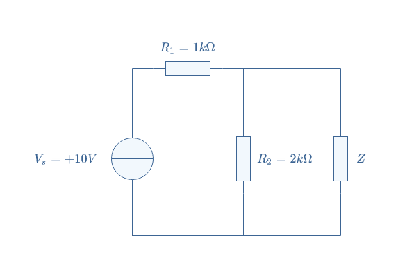
In order to determine the Norton model of this circuit, we remove the load Z and shorten the terminals of the circuit:

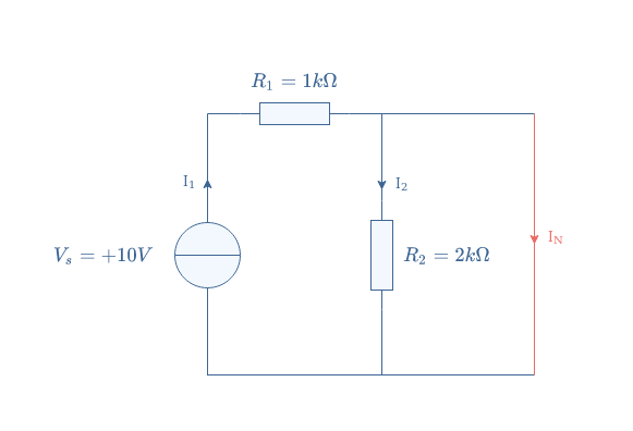
We can now determine the Norton current I_N, Kirchoff’s current law states that I₁=I₂+I_N. Since I_N does not cross any impedances, which means that the resistor R₂ is shortened, we can affirm that I₂=0.

Norton’s current is therefore equal to the current delivered by the voltage source, it can be computed by applying Kirchoff’s voltage law: V_s=R₁I₁+R₂I₂=R₁I₁ ⇒ I_N=V_s/R₁=10 mA.

To find Norton’s resistance R_N, we replace the voltage source by a wire:

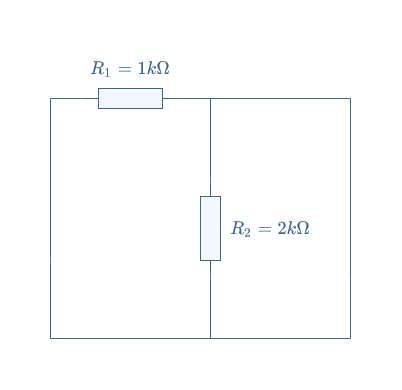
In this configuration, R₁ and R₂ are in parallel, the equivalent resistance is therefore given by R_N=(R₁×R₂)/(R₁+R₂)=666 Ω.

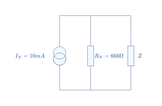
We can now give the Norton model of the circuit presented in Figure 4:

Single Current Source

We consider a similar example than in the previous subsection by replacing the voltage source by a current source:

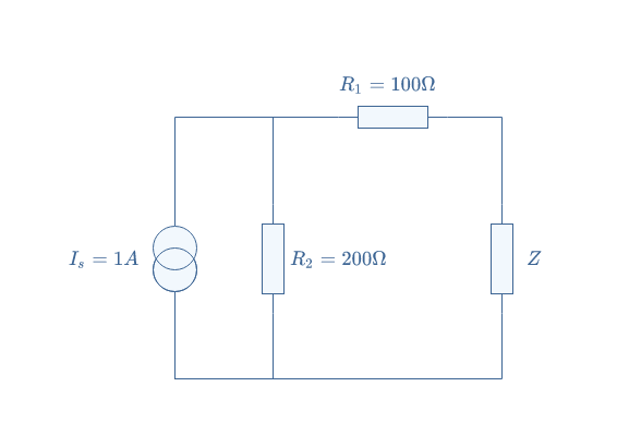
We proceed first by removing the load and shortening the terminals of the LEC. We label I₂ the current across the resistor R₂ and I₁=I_N the current across the resistor R₁. We simply find the Norton current by applying the current divider formula: I_N=(R₂/(R₁+R₂)×I_S=0.7 A.

We replace the ideal current source by an open circuit in order to find Norton’s resistance:

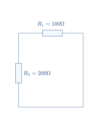
The equivalent resistance is simply given by the series associations R_N=R₁+R₂=300 Ω.

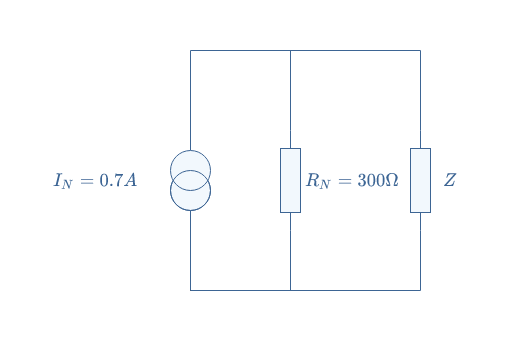
The Norton model of the LEC presented in Figure 6 is finally given by the following circuit:

Multi-current/voltage sources

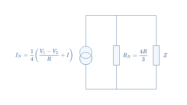
For the last example, we increase the complexity by including both current and voltage sources and more resistors in the same circuit. We consider the following LEC that we have already dealt with in our previous article concerning Thevenin’s Model:

We proceed again similarly by replacing the load Z with a wire in order to find Norton’s current. By applying Kirchoff’s current law, we get I=i₁+i₂+i₃+I_N. Moreover, by applying Kirchoff’s voltage law to every loop of the circuit, we get:

• i₁=i₂+V₁/R
• i₁=i₃-V₂/R
• i₁=I_N

After rearranging these equations to express I_N as a function of i₁, i₂, and i₃ in each line, we can finally isolate Norton’s current and find: I_N=(V₁-V₂)/4R+(I/4).

We have already demonstrated in the Thevenin theorem article that R_Th=4R/3 and since R_N=R_Th, the Norton resistance is thus already known.

Norton’s model of this complex circuit is given in Figure 9 below:

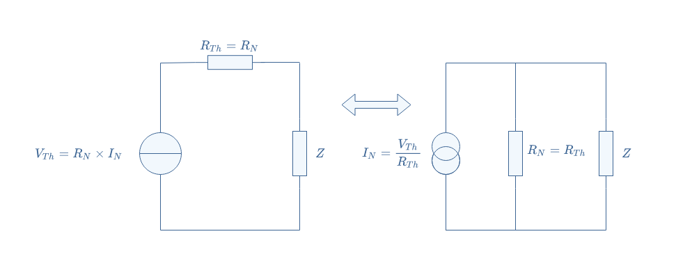
The link between Thevenin and Norton models

There is something very interesting to note about the multi-source example treated both in this article and the Thevenin tutorial. Indeed, if we proceed to the multiplication U=I_N×R_N, we find U=(RI+V₁-V₂)/3, it happens that this value is equal to the Thevenin equivalent voltage: I_N×R_N=V_Th.

From the knowledge of Norton’s parameter, we can, therefore, find Thevenin’s parameters for the same circuit: R_Th=R_N and V_Th=R_N×I_N. Reciprocally, the knowledge of Thevenin’s parameters can be converted into Norton’s parameters: R_N=R_Th and I_N=V_Th/R_Th.

The conversion between a Thevenin model to a Norton model or reciprocally lies only on one operation, we illustrate this conversion in Figure 10:

Conclusion

This tutorial has been built around one sentence, known as Norton’s theorem: “Any linear electrical circuit is equivalent to an ideal current source in parallel with an equivalent resistor“.

We have first presented the framework in which this theorem can be applied along with the definitions of some key concepts. We have seen that linear electrical circuits (LEC) consist of an interconnection of ideal sources and resistors. Ideal sources are well defined in the first section along with the equivalent resistance concept.

The second part is a short section that proposes a step-by-step method to follow in order to determine the Norton model of any LEC. The method is illustrated with real examples in a third section which proposes simple single-source circuits and finally a more complex architecture.

To conclude, we establish a link between Norton’s and Thevenin’s equivalent circuits by illustrating how to convert one model to another.

Please follow and like us: