Ohm’s Law

Introduction

The fundamental relation between the current, voltage, and resistance is known as Ohm’s law and is probably the most famous and elementary physical law of electronics. It is in 1827 when the German physicist Georg Simon Ohm publishes for the first time in the book “Die galvanische Kette, mathematisch bearbeitet” (in English: The mathematical study of the galvanic circuit) an early form of the law that will later take his name.

In the first section we will present the macroscopic Ohm’s law which is the form that is shown to students early in the learning process.

In the second section, we will see that different forms of the equation can be adapted depending on the topology of the circuit and the nature of its source, in particular when considering the AC regime.

More advanced concepts are presented in the third section where we focus on the mesoscopic definition of the equation which is known as the local expression of Ohm’s law.

Presentation

We consider an electric current I, flowing through a resistor R which produces a potential difference U at its terminals:

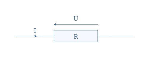
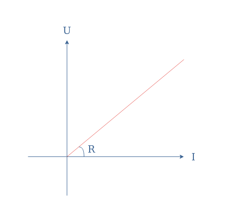
Ohm’s law establishes a simple linear relation between these three parameters such as U=R×I. Any electrical component that verifies Ohm’s law can be labeled as an ohmic conductor and presents a voltage-current characteristic such as presented in Figure 2:

It is important to note that Ohm’s law is empirical, meaning that it comes from experimental observations and not from a theory.

The macroscopic form is widely used in electronic circuits and it is a very useful formula to know. We can compute an unknown parameter (R for example) with the knowledge of two others parameters (U and I for example). Moreover, it allows us to write the expression of the dissipated power in a resistor under the form P=R×I².

Equivalence in AC regime

Ohm’s law can be generalized when the current and voltage are sine waveforms. In this case, we use the complex notation to write the law such as U=Z×I with Z being the complex impedance of a set of linear components (resistor, capacitor, and inductor).

In resistor

If we consider again the circuit presented in Figure 1 in AC regime, Ohm’s law can be written such as u(t)=Ri(t) with i(t)=I×sin(ωt), u(t)=U×sin(ωt+φ), and I, U being the amplitudes of the respective signals. However, since the phase difference in a purely resistive component is equal to zero, we obtain U=RI.

In inductor

Things get a little different when considering reactive elements, let’s begin with the inductor:

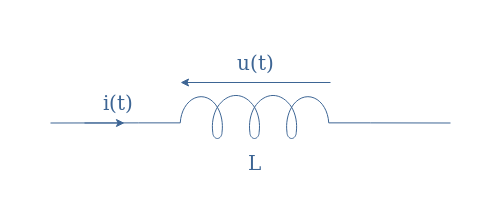
According to Lenz’s law, the voltage u(t) produced by an inductor is proportional to both the inductance and the variations of the current i(t) as shown in Equation 1:

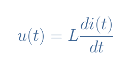
It can be shown from Equation 1 the relation between current and voltage can be written u(t)=Lω×Isin(ωt+φ). The demonstration is even easier when using the complex notation and knowing that the derivation operation in the complex domain is similar to multiplication by jω which consists in multiplying the phasor i(t) by ω and proceeding to a rotation of φ=+π/2 rad (see the tutorial about Phasors Diagrams & Algebra).

In an inductor, the current and voltage signals are therefore phase-shifted of Δφ=+π/2 rad. Since the voltage is usually considered to be the reference, its expression remains unchanged (u(t)=U×sin(ωt)), while the current can be written i(t)=I×sin(ωt+φ).

In capacitor

Finally, we consider a capacitor in the AC regime:

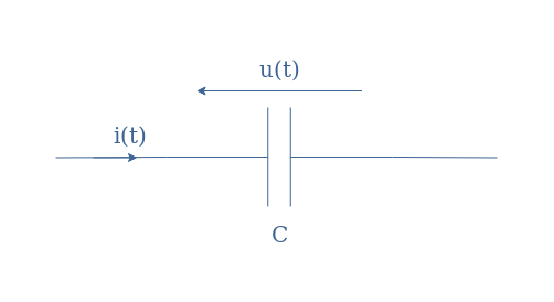
In this configuration, the charge of the capacitor is a function of time and its expression is q(t)=C×u(t). Since i(t)=dq(t)/dt, we can demonstrate directly or by using the complex notation that i(t)=-Cω×Usin(ωt+φ).

If we consider again the voltage to be the reference signal, the phase-shift is here Δφ=-π/2 rad, the expression of the current is, therefore, i(t)=I×sin(ωt-φ).

Local form

In this section, we discuss a more advanced concept known as the local form of Ohm’s law. Prior to presenting this special form, we need to introduce and define some concepts. We want to note that in the following, the vectors are bolded while the scalars are not.

Presentation and definitions

The local form can be applied to an intermediary scale of space between microscopic and macroscopic known as the mesoscopic scale. Typically, the mesoscopic scale is considered to be large enough to contain a large number of particles in an elementary volume (electrons in our case) but small enough so that the parameters such as the pressure and temperature stay local.

We usually refer to the electrons as “charge carriers” or simply “carriers”, they are defined by the carrier density n_e, their speed vector v, the elementary charge e, and their mass m_e.

From these parameters, we can define an important vector j known as the current density to be j=-en_ev. The term -en_e is also known as the charge density and noted ρ_e.

Drude model

Consider an ohmic conductor of section S submitted to a certain voltage V, this potential difference induces an electric field E which forces the carrier of the conductor to move:

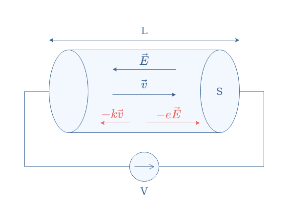
The movement of the carriers is dictated by two forces that act in opposite directions:

• The electrical force -eE tends to move the electrons in the opposite direction to the electrical field (same direction for positively charged carriers).
• A friction force -kv that tends to slow down electrons. This force is due to the motionless charges that constitute the crystal lattice of the ohmic conductor, which the electrons have a certain probability to crash in. The parameter k is a constant that depends on the material considered to be the conductor.

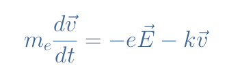
The Drude model (1900) consists of taking into account these two forces and apply the second law of Newton to the carriers:

Expression of the local form

We can rearrange Equation 2 and write k/m=1/τ with τ being the relaxation time parameter of the ohmic conductor:

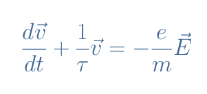
In permanent regime (t>>τ), this first-order differential equation accepts the following expression as a solution:

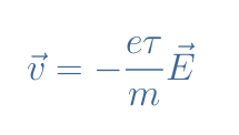
Finally, the current density can, therefore, be rewritten such as:

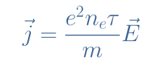
We usually write the scalar term σ which is known as the electric conductivity, the local Ohm’s law states that j=σE.

The local form is particularly helpful for studying the electrical properties at a microscopic scale.

Electric resistance and macroscopic Ohm’s law

The electric field in the ohmic conductor can be written E=(V/L)n with n being a unit vector in the same direction as E.

The electric current I is defined as:

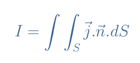
The current (C/s) can indeed be understood as the sum of the current density (C/m²/s) taken across the section (m²).

For the topology presented in Figure 5, the previous expression can be simplified to I=σES. When replacing the field E by V/L, we obtain:

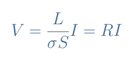
Finally, we can conclude that the local form of Ohm’s law enables us to retrieve both the macroscopic Ohm’s law and the definition of the resistance R=L/(σS). We can also note that 1/σ can be replaced by ρ which is defined as the resistivity of the ohmic conductor.

The simplification of the integral expression, however, appeals to two strong hypotheses: the conductivity σ is constant across the material and the current density j is colinear with the axis of the material and uniform. Basically, these two hypotheses can be gathered by assuming that the material is isotropic (uniformity in all orientations).

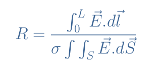
In the general case, for any topology and if the material is anisotropic, the resistance can be computed with the following formula:

Conclusion

This tutorial has focused on the famous physical law known as Ohm’s law. A recap is given in the first section where its framework, definition, consequences, and uses are shown.

The second section gives a more general form of the law where the supply source works in the AC regime. When considering the three elementary components of electronics, we realize that the form of the law in the AC regime does not change for the resistor but is written differently for the reactive components.

In the final section, we present the local form of Ohm’s law which is adapted for an intermediary scale between the macroscopic and microscopic world: the mesoscopic scale. Many new definitions and concepts are first introduced before explaining through the Drude model how to obtain the local expression. Finally, we demonstrate that the macroscopic form of the law along with the expression of the resistance can be retrieved from the local form.

Please follow and like us: