The Differential OPAMP Amplifier

Introduction

In the previous tutorials, we talked about the inverting op-amp and non-inverting op-amp, we considered configurations that take a single input on either pin “-” or “+” of the operational amplifier, while the other pin is grounded.

However, it is possible, as we will see during this article, to supply both inputs of an op-amp with signals in order to obtain an output that is directly proportional to the input difference. This new configuration is commonly known as a differential amplifier.

We introduce this new configuration in the first section where we present its functioning and demonstrate its output expression.

A simple example of a differential amplifier along with some basic differential-based applications is presented in the second section.

Finally, the last section briefly presents the instrumentation amplifiers which are essential differential-based configurations found in acquisition chains to treat sensor outputs.

Presentation

The goal of this section is to introduce the reader to the differential amplifier configuration and to demonstrate its output expression.

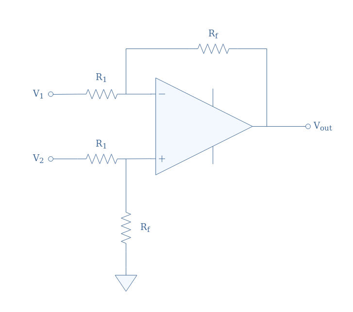
In Figure 1, we present the circuit representation of the basic differential amplifier. The inputs are labeled V₁ and V₂ and are in connection with the op-amp inverting and non-inverting pins through the resistors R₁ and R₂. The output is labeled V_out and the resistors R_f and R_g stand respectively for “feedback” and “ground”.

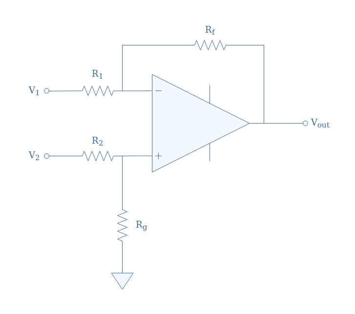
In the following, we will suppose the op-amp to be ideal, which is a very good approximation of modern real amplifiers. As a consequence, we have no currents entering through the pins – and + of the op-amp, moreover, the equality V₊=V_– between the potentials at the same pins is satisfied.

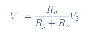
The voltage V₊ is determined by the voltage divider formula linking R₂ and R_g:

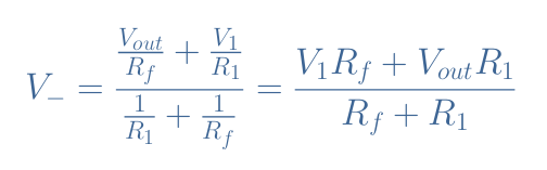
The voltage V_– can be written thanks to Millman’s theorem which stipulates that the potential at a node can be written as the sum of the currents entering the node and divided by the sum of the admittances in each branch:

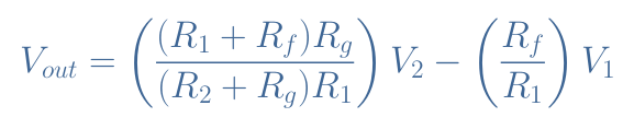
Since we suppose V₊=V_–, both previous equations are also equal. After rearranging this equality, we finally obtain the output expression for a differential amplifier in the general case, which is a superposition of both inputs V₁ and V₂:

Differential mode

The configuration R₁≠R₂≠R_f≠R_g is however never used in real circuits. What we should aim for when designing a differential amplifier is to get an output of the form V_out=A(V₂-V₁), with A being a common factor.

In the following paragraphs, we show under which condition (that we call differential condition) this common factor can be written.

In order to get a common factor for V₁ and V₂, the following equality must be satisfied:

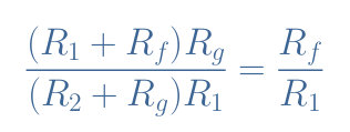
After some basic simplification steps, the differential condition can finally be written R_f/R₁=R_g/R₂. In this case, we obtain indeed V_out=A(V₂-V₁) with A=R_f/R₁.

We can even simplify the circuit by choosing R₁=R₂ and R_f=R_g (which still satisfies the differential condition and with again A=R_f/R₁):

Subtractor mode

If we add the conditions R₁=R_f and R₂=R_g, not only we satisfy the condition to write the output under the form V_out=A(V₂-V₁) but also we get A=1.

In this case, we cannot talk of the circuit as a differential amplifier since the difference V₂-V₁ is not amplified, we instead label the configuration as a subtractor with V_out being directly equal to the input difference.

Differential amplifier examples

As stated in the introduction, differential amplifier op-amps can be very useful to process the output signal of a sensor. We first present some very simple sensors that are resistors which resistance value depends on an external physical parameter.

In the second part, we need to present what is a Wheatstone bridge before focusing on the third part which deals with the integration of these sensors in a differential amplifier circuit to understand how the signal is processed.

Dependent resistor

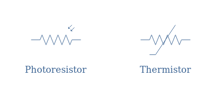
In the following, we present the basics of resistors which resistance values depend on the light intensity (photoresistor) or on the temperature (thermistor).

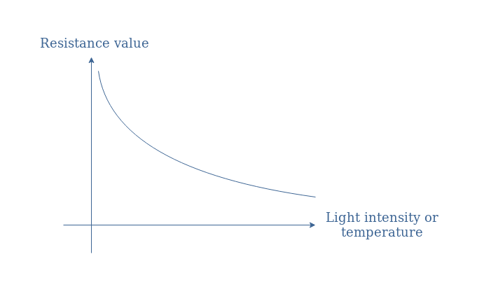
A good modelization for both photoresistor and thermistor resistance values is to consider an exponential decrease with an increase of the light intensity or temperature:

Wheatstone bridge

A Wheatstone bridge is a measuring circuit composed of 4 resistors interconnected in a loop configuration such as shown in Figure 5. One of the resistors has an unknown value (R_x), one is a variable resistor (R_v), and two have known and fixed values (R₁ and R₂).

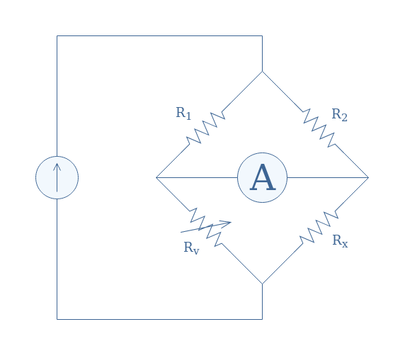
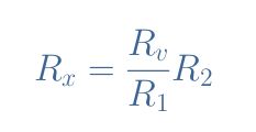
We won’t explain here the details about the measuring procedure of a Wheatstone bridge but we will assume that when no current is detected by the galvanometer (or amp meter) across the nodes R₁-R_v and R₂-R_x after adjusting the value of R_v, the resistance R_x is given by Equation 1.

This condition is also known as the balancing condition of the Wheatstone bridge.

Light/temperature detection

In the following Figure 6, we present a light-detection circuit based on a differential amplifier configuration, including a Wheatstone bridge with resistors R₁, R₂, the photosensitive resistor R_Ph which plays the role of the unknown resistor, and a light-adjusting resistor R_A which plays the role of variable resistor. The feedback resistor R_H adjusts the hysteresis.

Note that a temperature-detection circuit consists only of replacing the photoresistor by a thermistor.

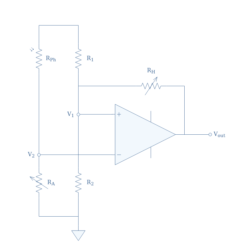
The goal of the resistance R_A is used to set the “reference” light-level, indeed, when a certain level of light changes the value of R_Ph, we can adjust R_A in order to balance the Wheatstone bridge and get a zero differential input V₂-V₁, and therefore no output signal as well.

When the light intensity changes, the circuit becomes unbalanced and a voltage difference V₂-V₁ appears. Even with a small luminosity change, the op-amp will amplify the differential signal in order to correctly detect it and eventually process it in the next stages of the circuit.

One possible way to process the signal is by connecting a LED to the output of the op-amp. The LED is only ON when the output voltage is above a certain value, it stays OFF otherwise. For the configuration presented in Figure 6, the LED would turn ON in the absence of light making it a “darkness detector”. To get the opposite effect and build a “light detector”, we simply need to exchange the positions of R_Ph and R_A.

Instrumentation amplifiers

One of the limitations of differentials amplifiers when it comes to process sensors outputs is its relatively low input impedance. Indeed, the input impedance of the general configuration presented in Figure 1 is equal to R₁+R₂, which is much lower than the input impedance of a common non-inverting op-amp.

In practice, for this reason, differential amplifiers are never used alone for processing sensor outputs as their low input impedance can bias what the source (sensor in our case) provides (see the tutorial op-amp building blocks for more information).

The solution to increasing the input impedance is to connect voltage followers before the inverting and non-inverting inputs of the differential amplifier. This configuration, known as an instrumentation amplifier, is presented in Figure 7 below:

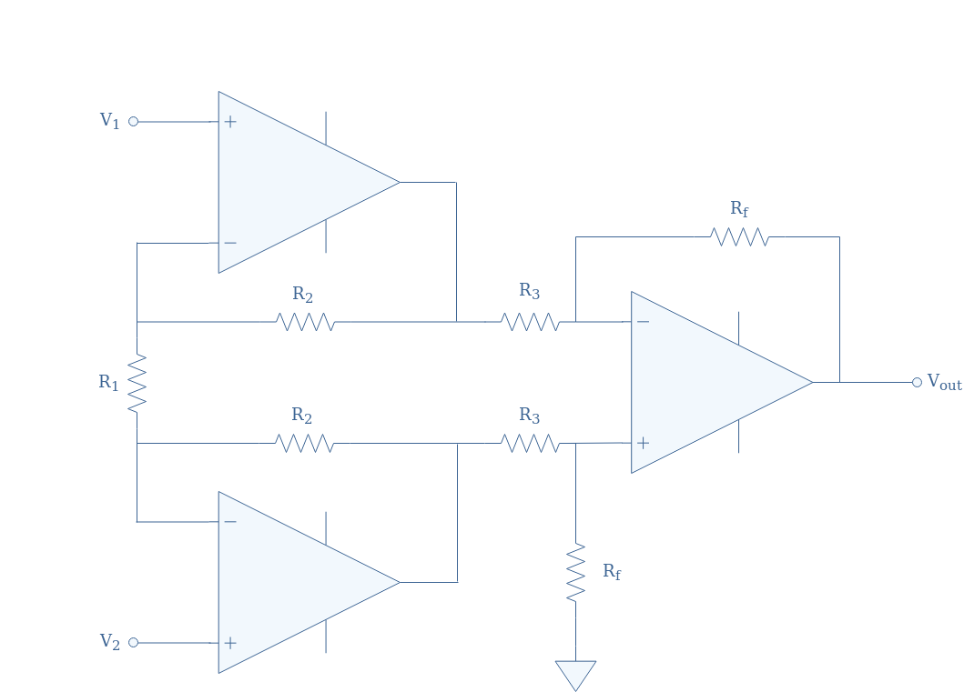
The voltage drop across the resistor R₁, which is the input of the differential amplifier, is equal to V₂-V₁, except that this time, the sources of the signals V₁ and V₂ sees a very high input impedance thanks to both buffers.

Conclusion

The primary goal of a differential amplifier is to amplify a voltage difference, that corresponds to the difference between the two input signals applied at its inverting and non-inverting inputs.

We have seen that in the general case (with arbitrary resistors), the op-amp doesn’t really amplify the difference since a difference factor is found for V₁ and V₂. It is actually more interesting to equalize the input resistances and the feedback and ground resistances (which we called the differential condition) in order to get an output of the form V_out=A(V₂-V₁).

In the second section, we dealt with a light/temperature detector circuit based on a differential amplifier. First, we briefly presented how a photoresistor/thermistor and Wheatstone bridge worked. The circuit shown in Figure 6 merges these different circuits and elements in order to create a simple light/temperature sensor.

However, the low input impedance that this circuit presents is its bigger disadvantage. In order to solve this problem, buffers are usually placed as an input to the differential amplifier as we present in the last section about instrumentation amplifiers.

Please follow and like us: